Reinforcement Learning 第四周课程笔记

• Temporal Difference Learning
• TD-lambda
• K-Step Estimators

本周三件事：看课程视频，阅读 Sutton (1988)，作业3（HW3）。

以下为视频截图和笔记：

Temporal Difference Learning

• Read Sutton, Read Sutton, Read Sutton. Because the final project was based on it!

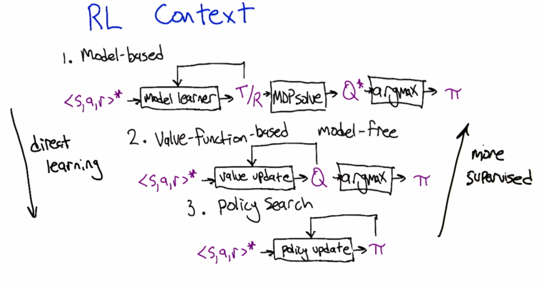
1. Model based
2. Model free
3. Policy search

• Form 1 –> 3: more direct learning
• From 3 –> 1 more supervised

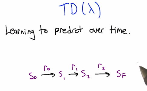
TD-lambda

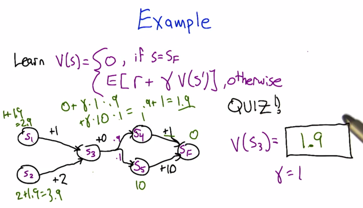
• in this case the model is known, the calculation is easy.

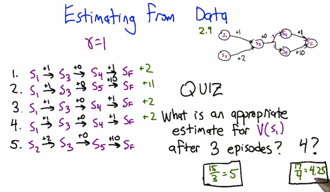
• Remember from the previous lecture, we need to get value from each episode and average over them.

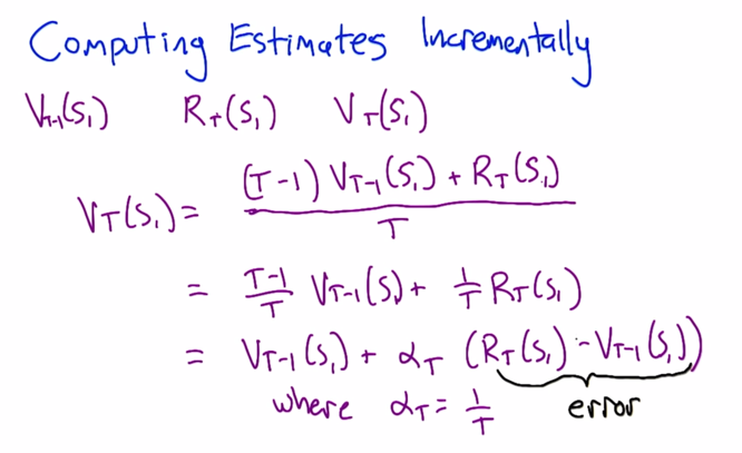
• The rewrite makes the formula looks a lot like neuro-net learning. and alpha is introduced.

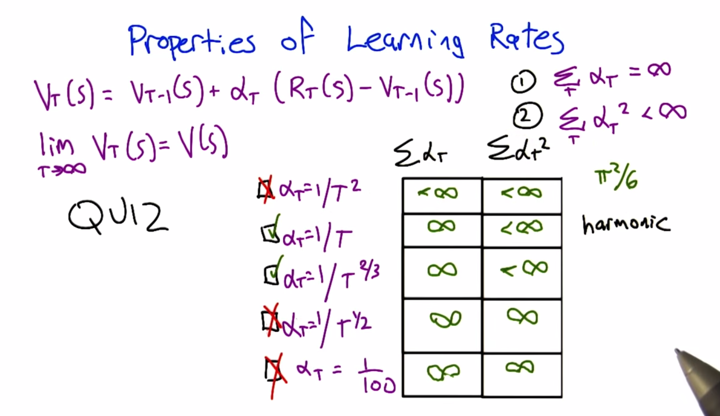
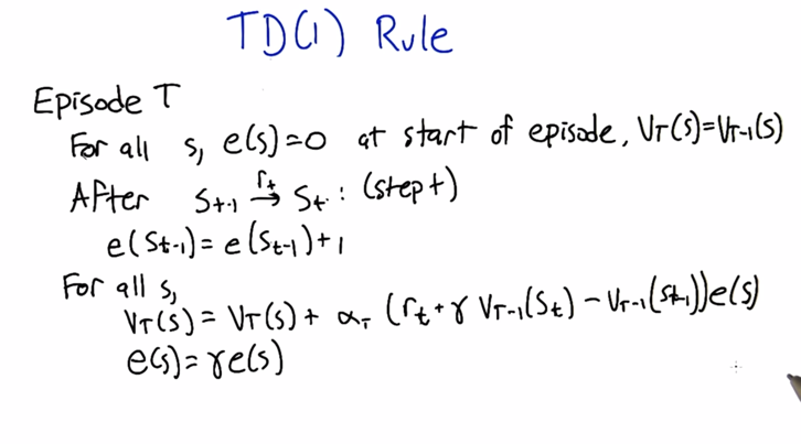
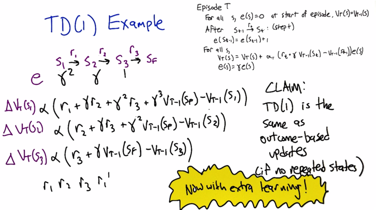
• When no repeated states, the TD(1) is the same as outcome-based updates ( which is see all the rewards in each state and update weights).
• when there is repeated states, extra learning happens.

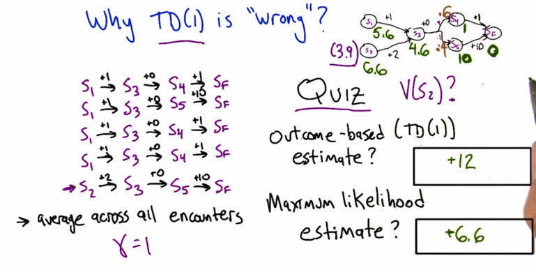
• in case of TD(1) rule, V(s2) can be estimated by average episodes. we only see V(s2) once and the value is 12. Then V(s2) = 12
• in case of Maximum likelihood estimates, we have to kind of learn the transition from data. e.g. for the first 5 episodes, we saw s₃->s₄ 3 times and s₃ -> s₅ 2 times. So the transition probability can be extracted from data as 0.6 and 0.4 respectively.

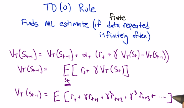
• First of all, if we have infinite data, TD(1) will also do the right thing.
• When we have finite data, we can repeatedly infinitely sample the data to figure out all the ML. This is what TD(0) do.

K-Step Estimators

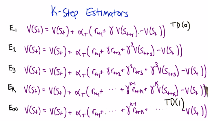
• E1 is one-step estimator (one-step look up) TD(0)
• E2 is two-step estimator, and Ek is k-step lookup.
• When K goes to infinity, we got TD(1)

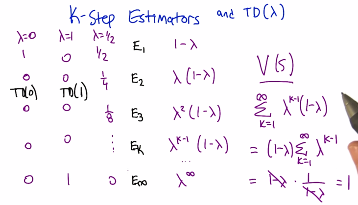
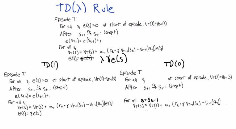
TD-lambda can be seen as weighted combination of K-step estimators. the weight factor are λ^k(1-λ).

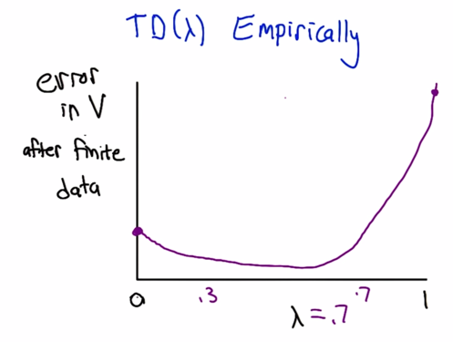
The best performed lambda is typically not TD(0), but some λ in between 0 and 1.

2015-09-5 初稿
2015-12-03 reviewed and revised until the "Connecting TD(0) and TD(1)" slides