Week 11: start Lesson 8, Pattern Rec Through Time (through New Observation Sequence for “We”), and read Chapter 15 in Russell & Norvig. Additional readings can be found on the course schedule.

Challenge question

given 2 HMMs, answer which model is more efficient to solve the problems in the quiz?

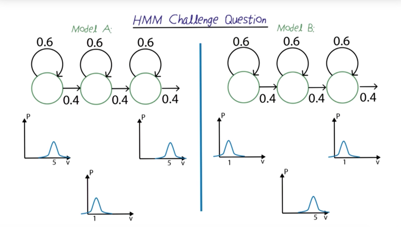
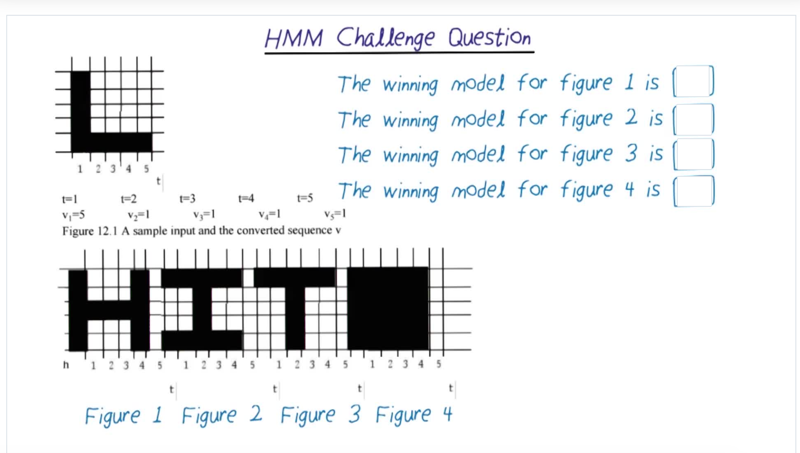
Answer is ABBA. A model expected high value at the first, low value in the middle and high value again at the end. B is opposite of A.

Dolphin Whistles

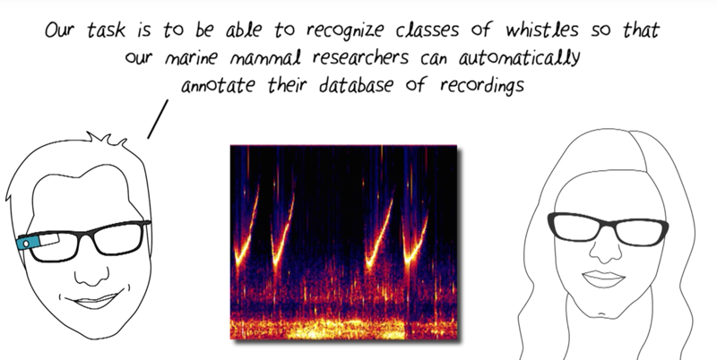
the figure is power spectrum of sound recording. The problem is to identify and match dolphin whistles in the data.

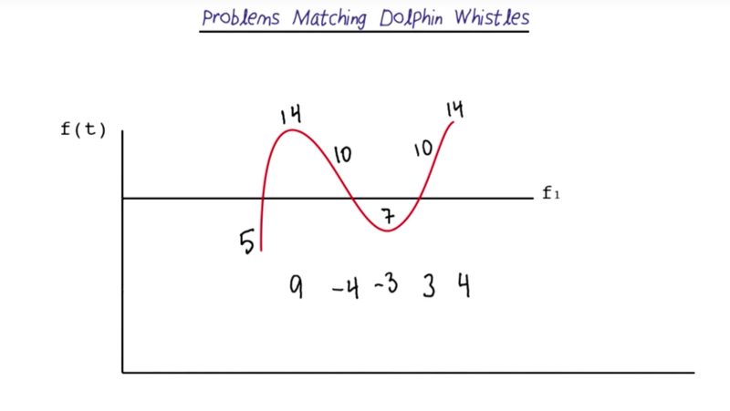
Problems Matching Dolphin Whistles

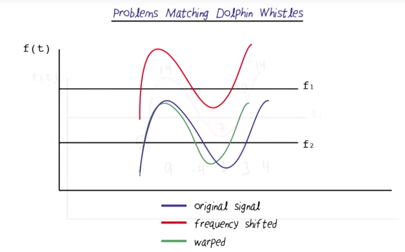
Frequency change up and down over time, so we can use delta frequency to represent the change

delta frequency

Warping Time

time warping

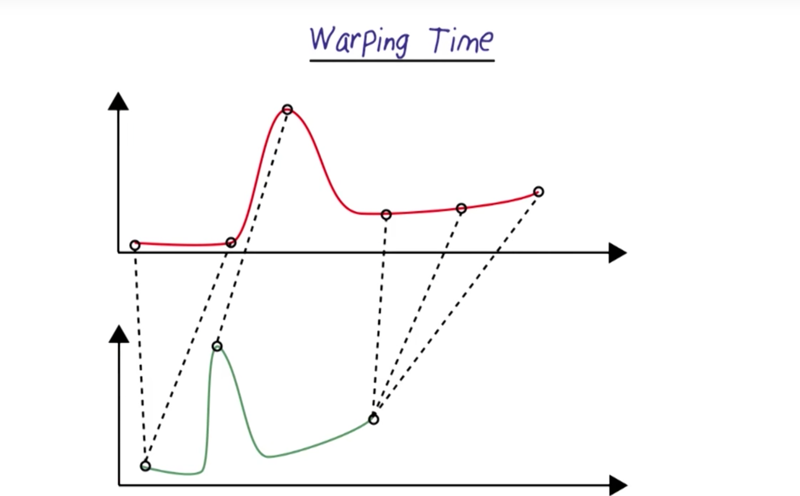
this is the problem to match features of the sound wave

Euclidean Distance Not Sufficient

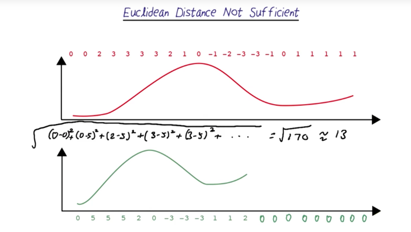
this method first zero-padding the short sound wave and then calculate the distance.

Dynamic Time Warping

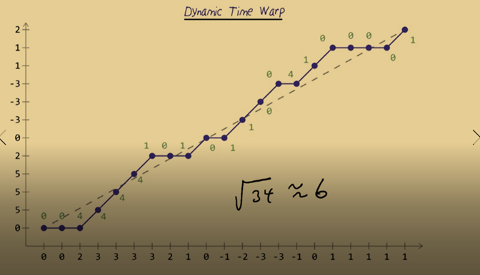
Dynamic time warping tries to align the samples between two whistles we’re comparing so that they best match up.
Plot the two whistles on a graph, one is on X-axis another is on Y. A match without any time warping would be a straight diagonal going from the lower left-hand corner to the upper right.
We match the long whistle to the short one. Start with the first sample in each signal. In this case, they’re both 0.
For the next sample in the x-axis, we have another 0. And it is better to stay matched to the 0 but not 5 because there will be less difference between 0 and 0 than 0 and 5. This procedure ensure minimization of distance.
After matching is done, then we can calculate the Euclidean Distance again and yield a distance about 6.

Sakoe Chiba bounds

problem with dynamic time warping

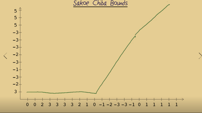
Dynamic time warping might be problematic for two signals that really are not that similar. The example in the above graph shows that the first a few cases in the X-axis have to match to 3 which makes the warping worse.

Sakoe Chiba Bound

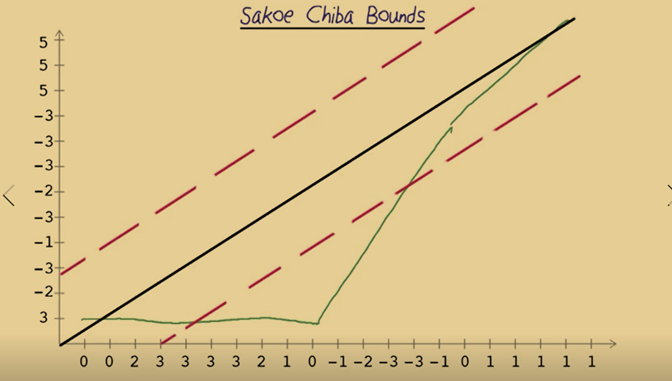
Sakoe Chiba Bounds can be applied so that the matching ends up with larger distance but match the shape more accurately. The idea is to apply bounds to the matching and then any matches outside the bounds would not be allowed. The bounds are empirically set by forming different bounds and select one through cross-validation.
The problem remains if different sections of the time series need different bounds. HMM can offer help on this.

Hidden Markov Models

HMM

Hidden Markov models, or HMMs as they’re known to their friends, are a useful tool for looking at pattern recognition through time.
They have states that represent a set of observed phenomena, and a set of transitions that describe how we can move from one state to another. What does “hidden” mean? - we don’t necessarily know which state matches which physical event. Instead, each state can yield certain outputs. We observe the output over time and determine a sequence of states, based on how likely they were to produce that output.
HMMs can codes sequences over time, we could use them for recognizing things like speech, handwriting or gesture or other time series data.
Techniques to improve HMM include state tiling, context, stochastic grammars and boosting.

HMM representation

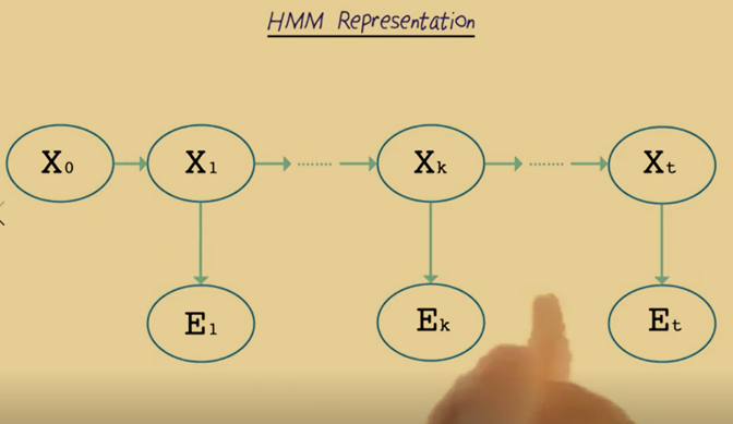
Traditional representation in ML world

The representation above is called Markov Chain which is common in the machine learning community.
Each Xi represents a frame of data. Xo is the beginning state which is useful for keeping data.X1 represents the first time frame t equals 1. E1 represents the output at that time.

Markov representation

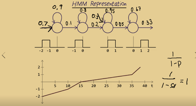
The graph above is made up of 4 different parts which can be represented by four states, from left to right and there is no looking back.
The four states can be represented by a boxcar.
The loops are called self-transitions, which indicates that the model can stay in the same state for several timeframes.
Alpha probabilities (emission probabilities): values that are allowable while we are in a given state. Note: these are not really probabilities since the output distributions are densities,
The first state has10 frames, the second has 5, the third has 20 and the forth have three. Thus, the probability of escaping state 1 and transiting to state 2 is then 1/10 = 0.1 and the probability of self-transition is 0.9. State 2 has 5 frames so its output probability is 0.2 and the self-transition probability is 0.8. The probabilities of other states can be defined this way too. Special case: if output probability is 1, then the transition will be guaranteed and no self-transition will happen.
Dummy state can be added before the initial state and the output of the dummy state represents the probability of entering the initial state (or state 1).

Sign Language Recognition

Example: sign language “I” and “we”. I is a gesture that First, the arm comes up towards the chest, and then pauses for a moment and then goes back down again. “we” is a gesture that the arm comes up toward to the right chest, pause a while, moves to the left horizontally, pause for a while and then goes back down.
The difference of the two gesture can be easily differentiated by delta X. but professor purposefully chooses to use the bad feature, delta Y, for the problem to demonstrate the power of HMM.

Quiz

Y and Delta-Y

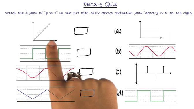
Given Y vs T, choose delta-Y vs t that matched it.
My answer is A, c, b, d, which is correct.

HMM for “I” and “we” gestures

HMMs

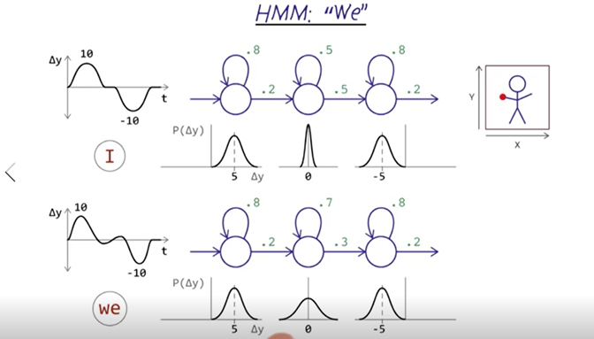
The graph above represents the “I” and “we” in HMM.
“I” State 1 is arm raising up, state 2 is a short pause and state 3 is arm dropping down. The probability can be represented by Gaussian.
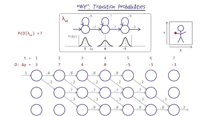
“We”: note that although there are four actions to complete the “we” gesture, from the point of delta-Y, there are only three states, and the only difference is that “we” stay in the middle state longer than “I”.

Quiz: what feature can help differentiating “I” from “we”?

features useful for the problem

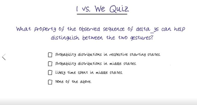
My answer will be the 2nd and 3rd options. And my answer is correct.

Viterbi Trellis

Vitrbi Trellis

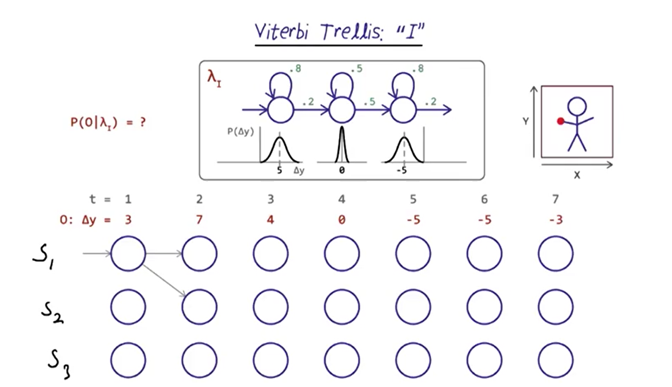
Viterbi trellis can show how likely each model generated the samples in O. The one that gives us the highest probability will be considered the proper match. The exact sequence of states that created the output is hidden, so we’ll need to go through all the possibilities.
when t = 1, delta-Y is 3, so it’s under the first Gaussian, and it can stay in state 1 or move to state 2 with the respective probabilities.
What’s the states could we in at t = 7 and t = 6 without considering the probabilities? The answer is chosen S3 for t = 7 and S2 or S3 for t=6 because we cannot jump from S1 to S3.

Nodes for “I”

Nodes for "I"

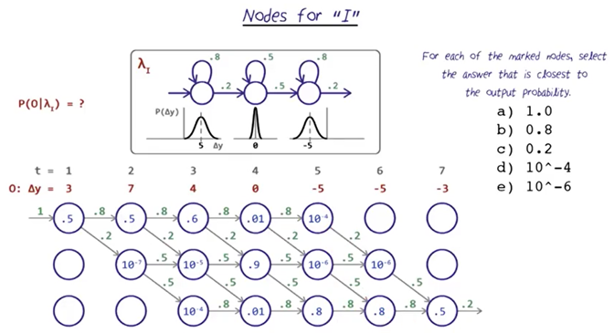
In the middle of the trellis it looks like we have many more options. We could really be in any of the three states.
Now we can fill in the transition probabilities. Which we can pull directly from our model, lambda I.

Viterbi Path

estimating Viterbi Path

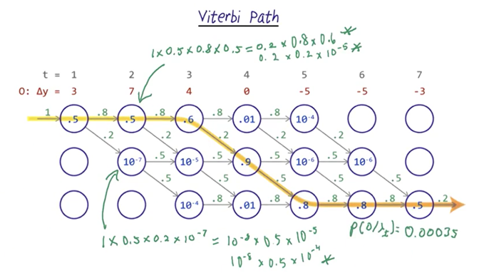
To establish the Viterbi path, we need to calculate the probability of each possible path and tract the paths which yield the best probability for each state. The final path was chosen based on the probability of output given lambda.
Note: the probability could be very small if we use the raw score, so in practice, the calculation usually uses log of the probabilities.
Now we can use the same procedure calculate the probability of output given lambda “we”.

nodes for “we”

Nodes for "we"

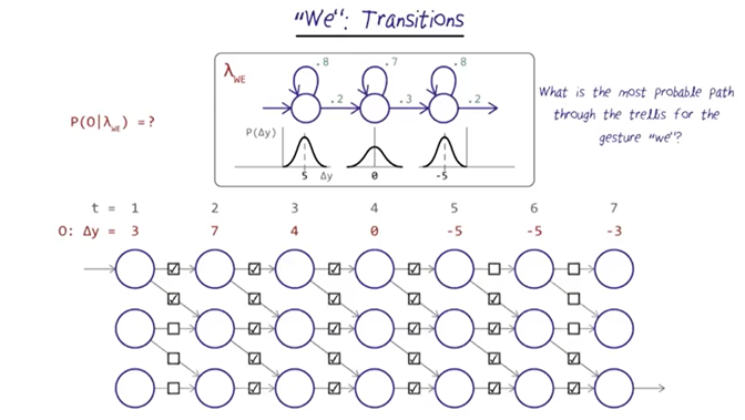
The procedure to calculate the probability of “we” and identify the Vertibi path is very similar to the “I” transitions.

First, identify the possible transitions ( which is the same as the “I” transition)

second

Second, fill in the transition probabilities for each state based on the model lambda “we”. And the main difference between the model for “we” and “I” are for the state 2.

third

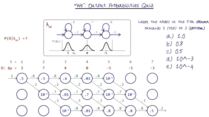
Third, fill in the output probabilities

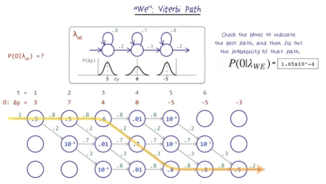
And last, figure out the largest expected probability and path (might or might not be the greedy path).
The path is the same as the “I” model, but the probability is much smaller.

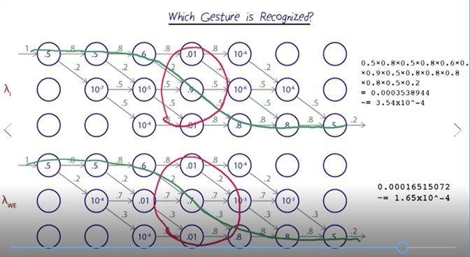
So it looks like it’s a lot more probable that the model for “I” generated this data. HMM can distinguish the tow gesture even when a relatively bad feature “delta-Y” is used.
The transition probabilities for the middle states reflect that with the gesture “I” spends much less time in the middle state than with “We”.
HMMs can appreciate is the accumulated difference in values over time for even relatively weak features

New observation for "I"

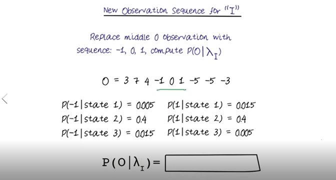
Given model for “I”, what’s the probability of the best Viterbi path?
The answer is 1.42 * 10^-5. Note: replacing 0 with a new sequence close to 0 actually increased the time of the second state.

New observation sequence for "we"

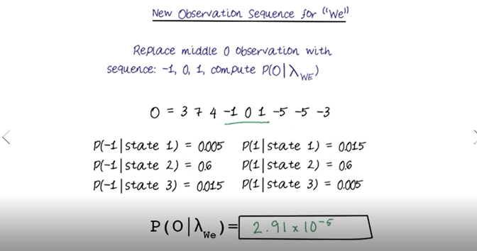
Now the same sequence gives the model for “we”, the probability increased to match “we” better. So the additional time in state 2 increases the probability of the gesture being “we”.

HMM Training

HMM Training from data

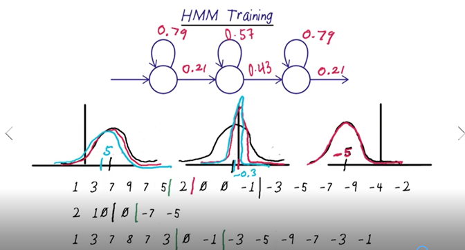
divide training sequences into 3 equal parts (corresponding to the number of states, which is 3 here)。
Estimate transition probability: calculate the average length of the sequence in the first states n1, then the transition probability will be 1/n1. Do this for the rest of the states. 3． Estimate the output distribution gave the data corresponding to the first state in all the training sequences. Calculate the mean and standard deviation from the data and use that to generate the expected Gaussian distribution. DO the same for all the other states.
Use the Gaussian distributions above to update the boundaries of each sequence.
With the new decision boundary and the classification of the members of each state to repeat 2 – 4 until converge, e.g. the decision boundary does not change anymore.
- What we’ve done so far is use Viterbi alignment to initialize the values for each state of our HMM. In other words, for each time frame in each of our examples, we’ve assigned a state it and calculated the resulting averages of all values assigned to each state along with the average amount of time we expect to stay in each state.

Baum Welch

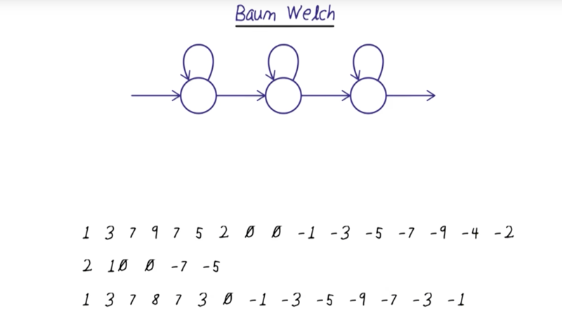
It’s very similar to Expectation-maximization but with Baum Welch, every sample of the data contributes to every state proportionally to the probability of that frame of data being in that state.
the calculation is a bit complicated but can use the forward-backward algorithm to help keep track of the calculations.

## Readings on HMMs

AIMA: Chapter 15.1-15.3

Rabiner’s famous Tutorial on hidden Markov models and selected applications in speech recognition [errata]

Thad Starner’s MS thesis: Visual Recognition of American Sign Language Using Hidden Markov Models[PDF]

The Hidden Markov Model Toolkit (HTK)

Please read Chapter 1 The Fundamentals of HTK (pages 3-13) in The HTK Book (version 3.4) [PDF HTML].

Multidimensional Output Probabilities

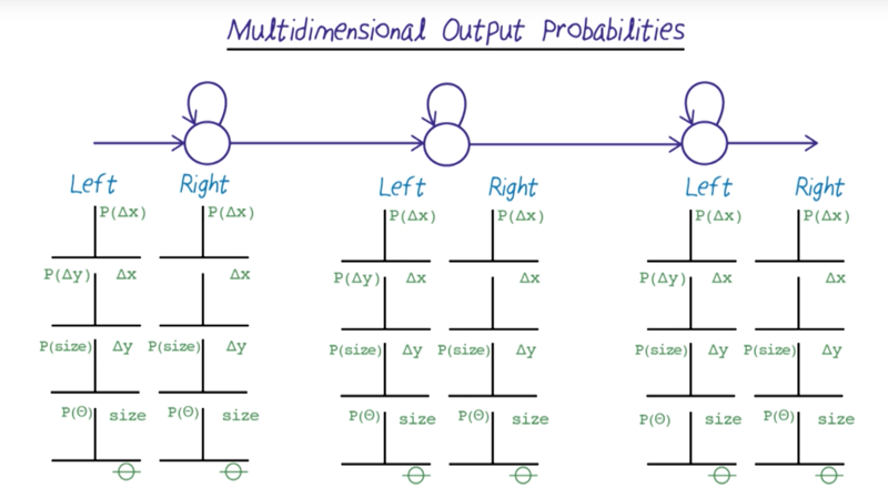
the sign language problem can have multiple features, e.g., x, y, size of hands, the angle of hands…, this will turn the problem into a multidimensional problem with 8 features.
calculate multi-dimensional distances

a mixture of Gaussian.

mixture Gaussian

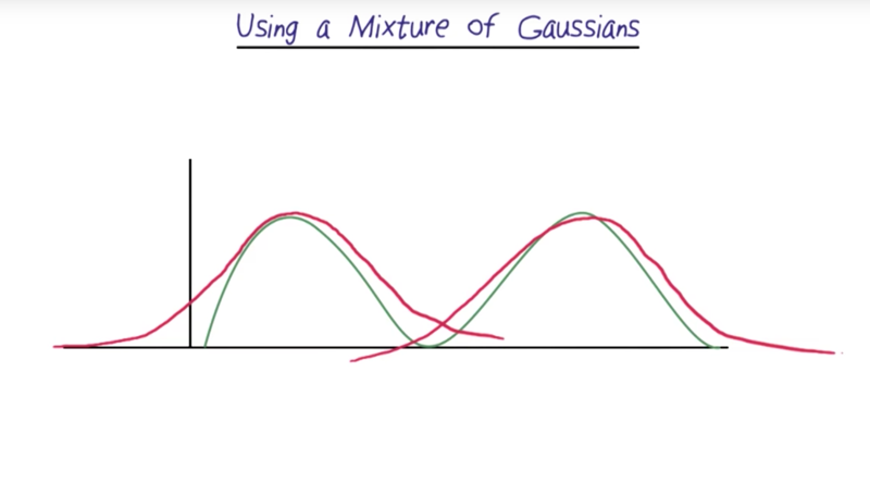
if output probabilities aren’t Gaussian, we can use a mixture of Gaussian to model it. In theory, any distribution can be modeled by a mixture of Gaussian.
The number of Gaussian needed depends on data. Limit mixtures to two or three Gaussians to avoid overfitting.

HMM Topologies

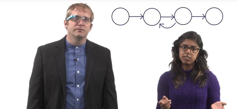
simple typology first and only add states when necessary.
for repeat stages, a loop can be added in the topology
In practice, we can try lots of different typologies, use cross-validation with randomly selected, training-independent test sets to settle on the best one.
the cat example: there are single-hand version and both-hand version. Solution: train separate model for both cases.

Phrase Level Recognition

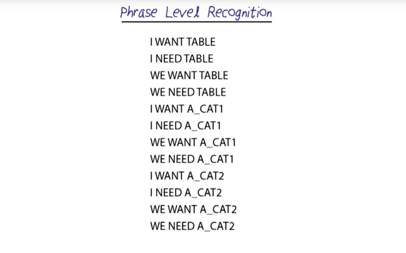
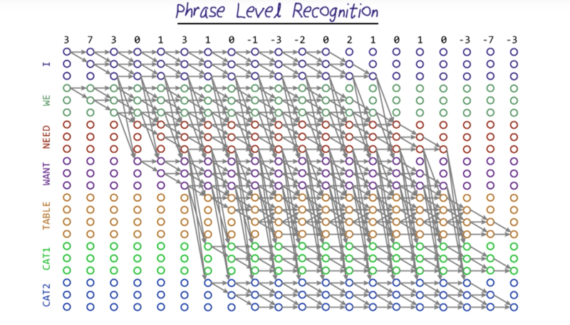
the algorithm is like a breadth-first search, expanding each possible path in each time step.
7 signs and 12 phrases.( two variants of cat we are recognizing) ordered by grammar sequence.
using delta y as a feature, we can get the graph above which shows the probability in each time point.
most all of language recognizers will have problems keeping the full trellis and memory. And keeping all the paths updated will also be a problem.

Stochastic Beam Search

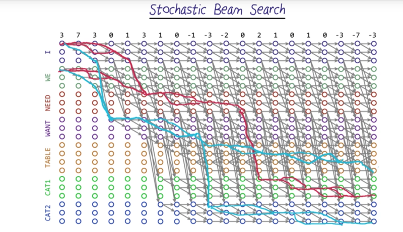
Now with Stochastic Beam Search, we can prune the “search” by dropping low probability paths. But we don’t want to get rid of all the low-probability paths. It is possible that there is a bad match in the beginning of the phrase that becomes a good match later on.
keep the paths randomly in proportion with their probability. (like the fitness function in Genetic Algorithm)

Context Training

Train several signs together

exmple of 2-sign complex

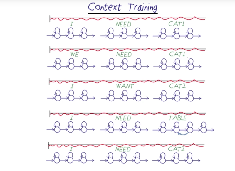
context training can divide our error rate in half.
In speech, the effect of one phoneme affecting the adjacent phoneme is called coarticulation, and this method of modeling the phrases is called context training.
signs in phrases of signs are different to isolated signs, the combination of movements looks very different. Solution: Train on phrases of sign.
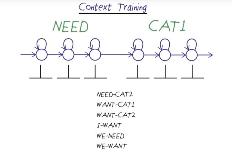
Method: dividing the data for each state in each sign; iterating and adjusting the boundaries of each state and each sign until convergence. Then find every place where I NEED occurs and train on the six-state model. ( fewer combinations are available).
The output probabilities at the boundary and the transition probabilities in between the boundary will be tuned to better represent the combination
Why not use three sign contexts? A: there might not be enough context to support this training.

Statistical Grammar

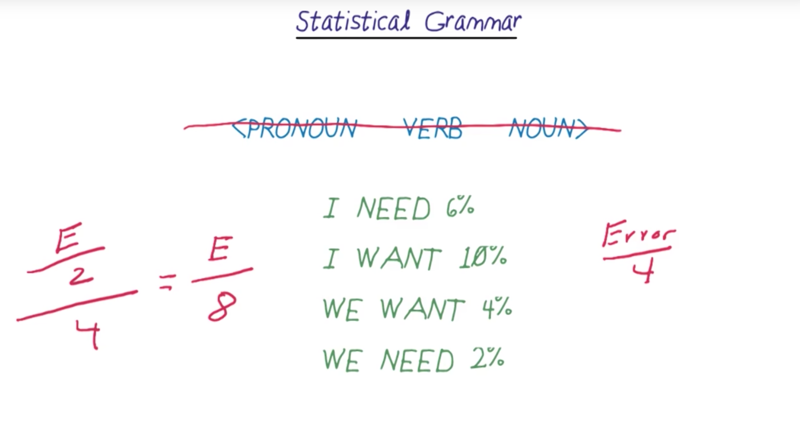
Statistical grammar places a strong limit of where we started and ended in our Viterbi trellis.
In practice, using a statistical grammar divides the error rate by another factor of 4.

State Tying

State Tying means combining training for states with the states within the model are closed.
For example, the initial state and the end state of “i” and “we” signs are very similar, so they can be trained together.
with Context training, things become complicated because the initial and end states are the states of complex and they are the first state of the first sign and the last state of the last sign.

HMM Resources

AIMA: Chapter 15.4-15.6 (provides another viewpoint on HMMs with a natural extension to Kalman filters, particle filtering, and Dynamic Bayes Nets), Chapter 20.3 (hidden variables, EM algorithm)

Further study

Huang, Ariki, and Jack’s book Hidden Markov Models for Speech Recognition.

Yechiam Yemini’s slides on HMMs used in genetics (gene sequencing, decoding).

Sebastian Thrun and Peter Norvig’s AI course:

HMMs and Kalman filters

Natural Language Processing

Natural Language Processing II

Segmentally Boosted HMMs

SBHMMS

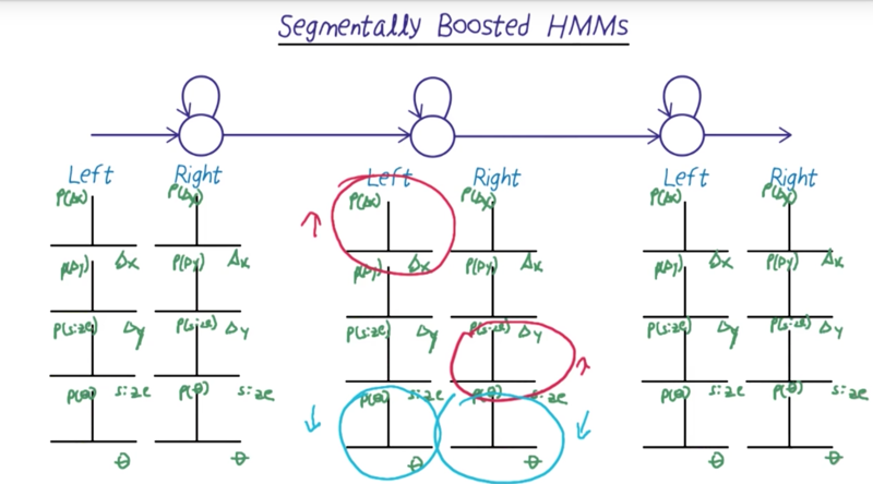
How SBHMMS work? A: First, we align and train the HMMs as normal. Next, we use that training to align the data that belongs to each date as best we can. We examine each state in each model iteratively and boost by asking which features help us most to differentiate the data for our chosen state versus the rest of the states. We then weight the dimensions appropriately in that HMM.
the method is useful to combat the problem of noisy dimension.
This trick combines some of the advantages of the discriminative models with generative methods.

Resources for Segmentally Boosted HMMs

SBHMM project at Georgia Tech

HMM Tool Kit (HTK)

Gesture and Activity Recognition Toolkit (GART; formerly Georgia Tech Gesture Toolkit)

Further study

Pei Yin’s dissertation: Segmental discriminative analysis for American Sign Language recognition and verification

Using HMMs to Generate Data

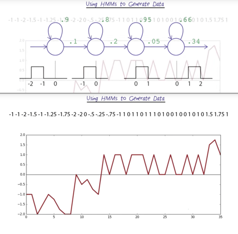
Using HMMs to Generate Data is not a good idea
the output distributions have no idea of continuity.
We could use a lot of states to try to force a better ordering of the output, but that would lead to over-fitting.

HMMs for Speech Synthesis

Junichi Yamagishi’s An Introduction to HMM-Based Speech Synthesis

Heiga Zen’s Deep Learning in Speech Synthesis

DeepMind’s WaveNet

初稿 2017-12
修订发布 2018-09-23

AI 笔记 Week 11-12 Pattern Rec Through Time