• 01-02 - Are you ready
  • Lesson outline
  • 03 - Global statistics
  • 04 - Compute global statistics
  • 05 - Rolling statistics
  • 06 - Quiz: Which statistic to use
  • 07 - Bollinger Bands
  • 08 - Computing rolling statistics
  • 09 - Quiz Calculate Bollinger Bands
• 10 - Daily returns
• 11 - Quiz Compute daily returns
• 12 - Cumulative returns

01-02 - Are you ready

Lesson outline

Pandas makes it very convenient to compute various statistics on a dataframe:

• Global statistics: mean, median, std, sum, etc. [more]
• Rolling statistics: rolling_mean, rolling_std, etc. [more]

You will use these functions to analyze stock movement over time.

Specifically, you will compute:

• Bollinger Bands: A way of quantifying how far stock price has deviated from some norm.
• Daily returns: Day-to-day change in stock price.

03 - Global statistics

• mean of each of these columns df1.mean()
• mean, median, standard deviation, sum, prod, mode…( at least 33 global statistics) can be computed in this way.

Global statistics: mean, median, std, sum, etc. [more]

Time: 00:01:15

04 - Compute global statistics

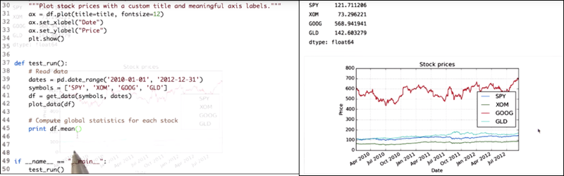
df.mean() returns mean of stock prices for each symbol. df.median() returns median of stock prices for each symbol. df.std() returns standard deviation. Mathematically, the standard deviation is the square root of the variance.

Time: 00:01:53

05 - Rolling statistics

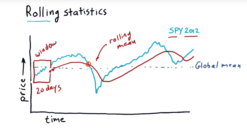
• Rolling statistics, take a sort of a snapshot over windows of time and calculate statistics.
• Global mean: compute the statistics across the whole period of time.
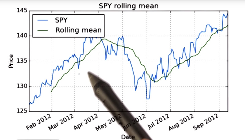
• 20-day rolling mean: take the mean of all that data in-between a 20-day window. (the little box in the graph). Then move the window forward one-day and take another mean, and so on. do that every day over this entire year, the rolling mean is the red line in the graph.
• We could do standard deviation, mode, median and so on.
• Technical indicators: rolling statistics can be used as technical indicators of the market.
• hypothesis: rolling mean may be a good representation of sort of the true underlying price of a stock, and those significant deviations from the rolling mean result in a return to the mean. The challenge is to know when is that deviation significant enough to be treated as buying opportunity…

Time: 00:03:06

06 - Quiz: Which statistic to use

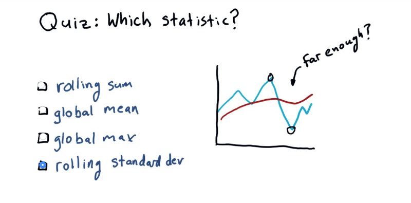
Given a rolling mean (in red), and the price in blue. what statistics to use to look for a buy signal or a sell signal. In another word, how can we decide that we’re far enough away from the mean that we should consider taking actions?

Rolling statistics: rolling_mean, rolling_std, etc. [more]

Time: 00:00:36

07 - Bollinger Bands

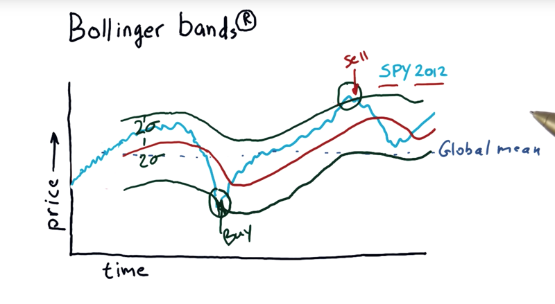
• Bollinger Bands: 2 standard deviations above and below the rolling mean is the Bollinger Bands.
• if the stock price falls out of the Bollinger Bands, you should pay attention. when the price comes back into the band, it is likely an opportunity to take action to buy and sell. (Real stock Market is not that simple, don’t take this and start trading!!!)
• Note: the professor is not necessarily endorsing technical analysis here. But he thinks “it can be very powerful”.

Time: 00:02:49

08 - Computing rolling statistics

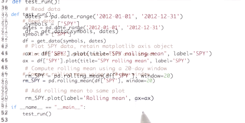
rm_SPY = pd.rolling_mean(df['SPY'], window=20) is the line calculate the rolling mean. the rest of the cold is to plot the rolling mean and the stock prices together.

• Next we call the rolling mean function from pandas library and pass in two parameters. The first parameter is the values for which the rolling mean has to be calculated. The next parameter is the window size, we use a period of 20 days.

• For working with time series data, pandas provide a number of functions to compute moving statistics.

• Observe that the rolling mean has missing initial values. For window size = 20, so the first 20 days there are no values.

Time: 00:02:07

09 - Quiz Calculate Bollinger Bands

It’s quiz time. 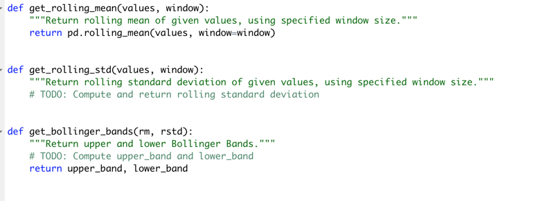Implement the functions to calculate rolling bands.

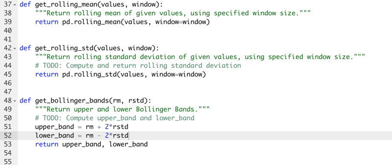
• Note: at the time that I am taking the course, pd.rolling_mean(), pd.rolling_std() is being deprecated.

  Errors:-

  • FutureWarning: pd.rolling_mean is deprecated for Series and will be removed in a future version, replace with Series.rolling(window=10,center=False).mean()
  • FutureWarning: pd.rolling_std is deprecated for Series and will be removed in a future version, replace with Series.rolling(window=10,center=False).std()

Time: 00:01:17

10 - Daily returns

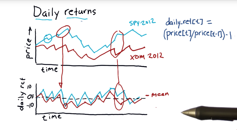
• Daily returns are one of the most important statistics used in financial analysis.
• Daily returns are simply how much did the price go up or down on a particular day
• Daily return = (price[t]/price[t-1]) - 1, where t is “today” and t - 1 is “yesterday”
• Daily return is a line that sort of zigs and zags, usually close to zero. the mean would probably be a little bit positive, above zero.
• looking at daily returns between different assets, can be revealing.

Time: 00:03:11

11 - Quiz Compute daily returns

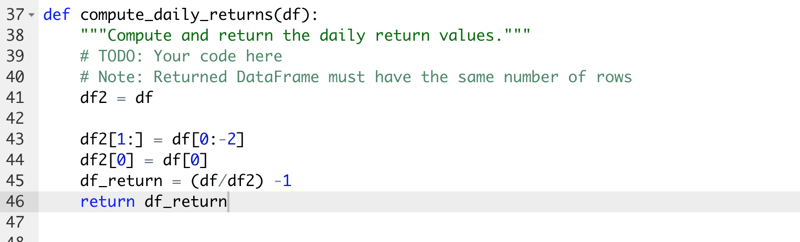
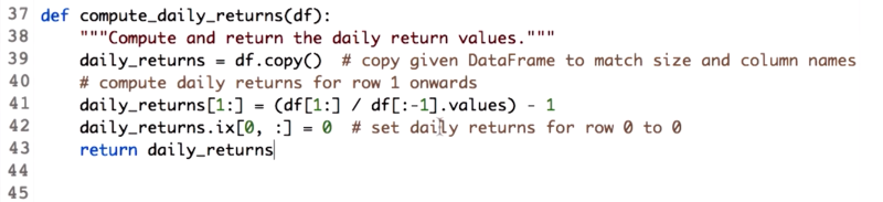
• when create new df, use df1 = df.copy()
• .values attribute is necessary because when given two data frames, Pandas will try to match each row based on the index when performing element-wise arithmetic operations.

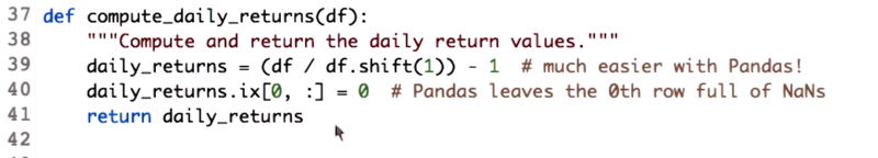
• using Pandas data frame function, shift.

Time: 00:02:25

12 - Cumulative returns

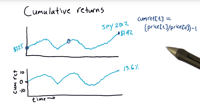
• the equation is CumRet[t] = (price(t)/price[0]) - 1
• The cumulative return for a particular day, t, is just today’s price divided by the price at the beginning.
• the equation is essentially a normalization.

Time: 00:02:22

Total Time: 00:23:17

First draft: 2019-01-11