01 - Overview

This lesson shifts now to computing statistics on portfolios.

a portfolio is an allocation of funds to a set of stocks. assume the allocations sum to 1.0.
we’re going to follow a buy-and-hold strategy and observe how things go moving forward.

Time: 00:00:36

02 - Daily portfolio values

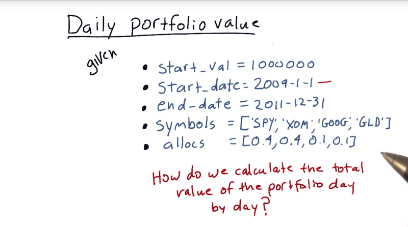
an example portfolio value of one million dollars. from the beginning of 2009 to the end of 2011.

And our portfolio with three symbols, S & P 500, Exxon, Google, and Gold. initial allocation: 40% -> SPY, 40% -> Exxon, 10% -> Google, and 10% -> Gold, and hold them. How do we calculate the total value of the portfolio day by day?

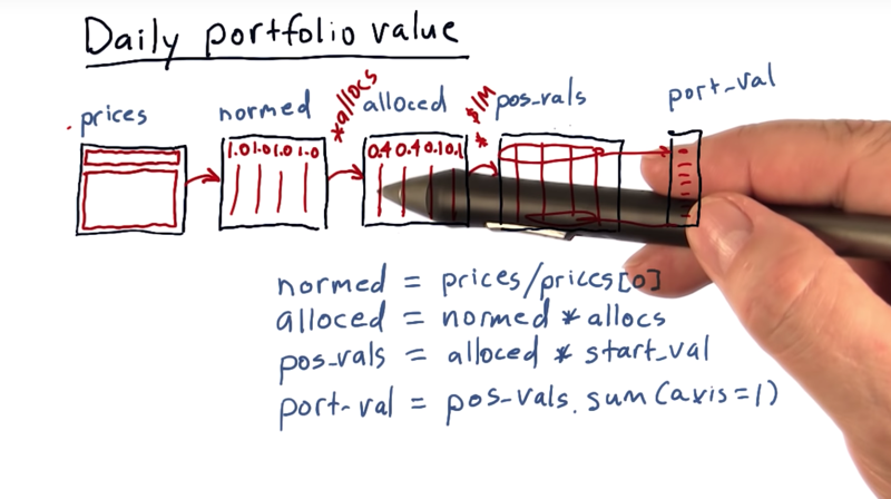
The first step is to normalize these prices by the first row. and get normed values
The next step is to multiply these normed values by the allocations to each of the equities. -> new data frame alloced.
the next step is to multiply our alloced data frame times start_val. then get in this first row the amount of cash allocated to each asset and then going forward, it’ll show us the value of that asset over time. (pos_vals),
Now summing pos_vals across each day and get port_val
Now those values change of course as the stock prices change going forward.

Let’s recap now.

We start with our prices.
We normalize that to the first day, so the first row here is all ones.
We multiply it times our allocations, and that gives us now in each column, the relative value of each of those aspects over time.
We multiply by our initial investment, and that causes now each row to be the real value of that investment each day over time, starting with our initial allocations.
If we then sum each row we get the value of the portfolio on each corresponding day, and that’s it.

Time: 00:04:37

03 - Portfolio statistics

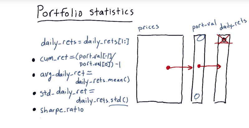
After we got from prices to port-val, we can compute a number of important statistics on the portfolio to the portfolio and the investment style of the portfolio manager.

first, compute daily returns and remove the first value because it is always 0 since on the first day there’s no change.

Four key statistics to evaluate the performance of a portfolio.

cumulative return, port_val[t]/port_val[0] - 1
average daily return, daily_returns.mean()
standard deviation of daily return: daily_returns.std()
sharp ratio.

Time: 00:02:03

04 - quiz: Which portfolio is better

The idea for Sharp ratio is to consider our return or our rewards in the context of risk.
risk: be standard deviation or volatility.

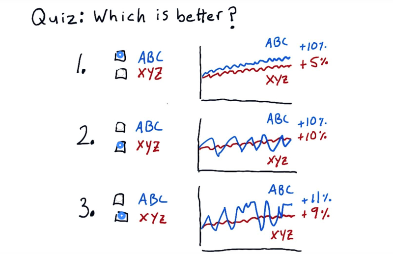
mark which portfolio or stock you think is better in each one of these examples.

Solution:

ABC is the correct answer because its volatility is the same but its total return is higher.
the correct answer is XYZ. is had the same return as ABC, but it was less volatile.
no enough information to make the choice here.

we need a qualitative way, Sharpe ratio, to measure this

05 - Sharpe ratio

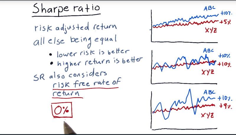
Sharpe ratio is a metric that adjusts return for risk.
it considered 1) risk, 2) return and 3) risk free rate of return when evaluating a portfolio.
the risk free rate of return is the interest rate you would get on your money if you put it in a risk free asset like a bank account or a short term treasury.
The Sharpe ratio is developed by William Sharpe

Time: 00:02:05

06 - Quiz Form of the Sharpe ratio

Consider Portfolio return (higher is better), risk-free rate of return (), and standard deviation of portfolio return, or volatility, or risk (lower is better). How would you combine these three factors into a simple equation to create a metric that provides a measure of risk adjusted return?

Solution

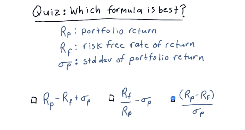
The solution above is indeed the form of the sharp ratio.

Time: 00:00:47

07 - Computing Sharpe ratio
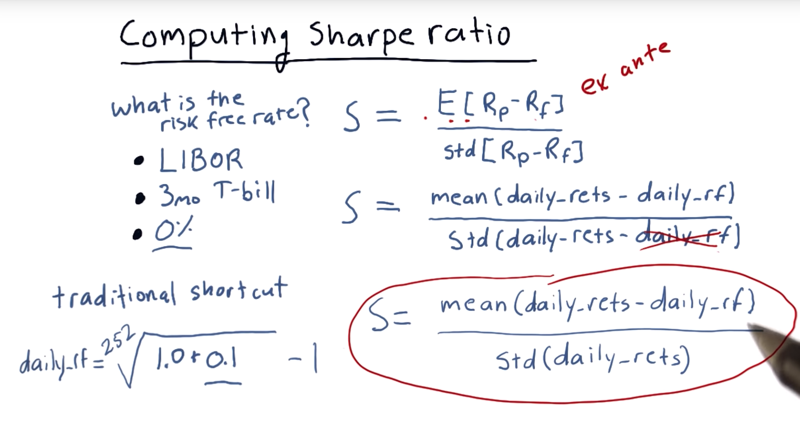
William Sharpe’s equation S=E[R_p - R_f] / std[R_p - R_f]. Here R_p if portfolio retern rate, R_f is risk free return rate.
R_f usually have three sources
1. LIBOR (the London Interbank Offer Rate).
2. interest rate on the 3-month Treasury bill
3. 0%
4. traditionally, there is a shortcut: the 252nd root of annual interest rate minus 1.
Note: When R_f is a constant, it can be removed from the std() function. So, S= mean(daily_returns - daily_rf)/std(daily_returns)

Time: 00:03:59

08 - But wait, there’s more

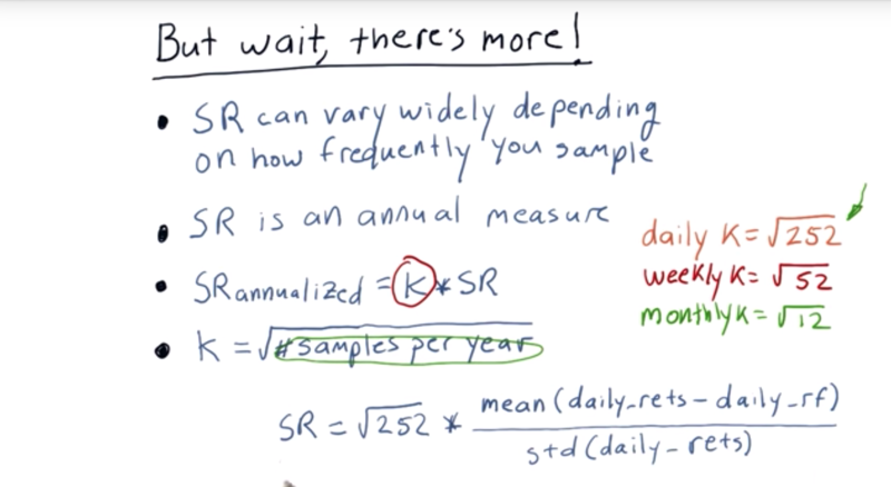
Sharpe ratio for the same asset can vary widely, depending on how frequently you sample it.
So there is an adjustment factor K developed to deal with this. K is related to the sample rate, so we have K_daily, K_weekly, K_monthly.
- K_daily = sqrt(252)
- K_weekly = sqrt(52)
- K_monthly = sqrt(12)
Note, if the data is daily data, even we only traded for 89 days, we still use sqrt( 252 ) as K, since we’re sampling daily.
Bringing it all together, the Sharpe ratio needs to be adjusted for the data samply rate

Time: 00:02:20

09 - What is the Sharpe ratio

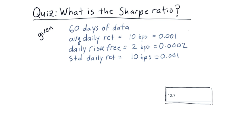
What is the Sharpe ratio of this strategy?

Recall the formula for computing Sharpe ratio:

k * mean(daily_rets - daily_rf) / std(daily_rets) where k = sqrt(252) for daily sampling.

Time: 00:00:42

Time: 00:01:05

10 - Putting it all together

Recap: we learned how to compute daily portfolio values and, from there, important portfolio statistics.

1) cumulative return, 2) average daily return, 3) standard deviation of daily return, or risk, and 4) Sharpe ratio.

Time: 00:00:33

Total Time: 00:21:43

2019-11-13 初稿

ML4T 笔记 01-07 Sharpe ratio and other portfolio statistics