- This week’s tasks
- Why changing RF?
- How to change RF without changing optimal policy.
- Q-learning with potential
- What have we learned?
This week’s tasks
- watch Reward Shaping.
- read Ng, Harada, Russell (1999) and Asmuth, Littman, Zinkov (2008).
- office hours on Friday, October 2nd, from 4-5 pm(EST).
- Homework 6.
Why changing RF?
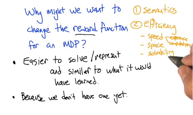
Given an MDP, RF can affect the behavior of the learner/agent so it ultimately specifies the behavior (or policy) we want for the MDP. So changing rewards can make the MDP easy to solve and represent
- Semantics: what the agent are expected to do at each state;
- Efficiency: speed (experience and/or computation needed), space (complexity), and solvability .
How to change RF without changing optimal policy.
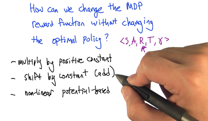
Given an MDP described by <S, A, R, T, γ>, there are three ways to change R without changing optimal solution. (Note, if we know T, then it is not a RL problem any more, so this part of lecture if for MDP not RL specifically).
- Multiply by a positive constant ( non-zero ‘cause multiply by 0 will erase all the reward information)
- shift by a constant
- non-linear potential-based
1. Multiply by a positive constant
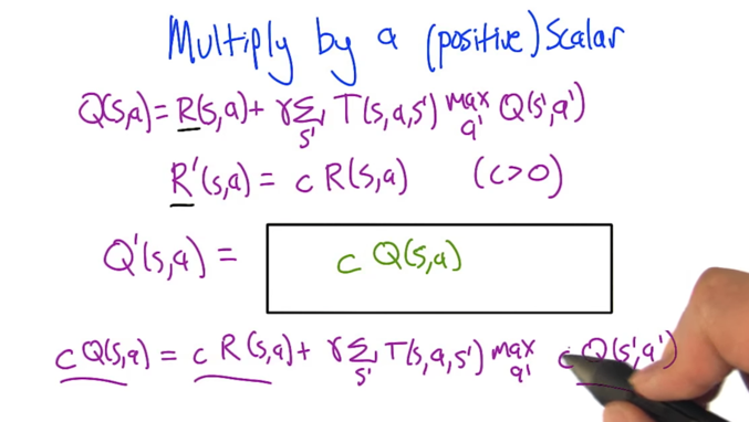
- Q(s,a) is the solution of Bellman function with the old RF R(s,a).
- R’(s,a) is a new RF with is the old RF multiplying by a constant.
- What’s the new solution Q’(s,a) with respect to the new RF R’(s,a) and old Q(s,a)?
Here is how to solve the problem:
- Q = R + γR+γ2R + … + γ∞ R)
- Q’ = R’ + γR’+γ2R’ + … + γ∞ R’
- Replace R’ with c*R, Q’=(c*R) +γ(c*R)+γ2(c*R) + … + γ∞ (c*R) =c(R + γR+γ2R + … + γ∞ R) =c*Q
2. shift by a constant
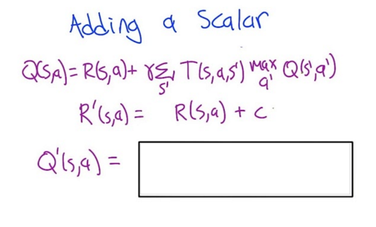
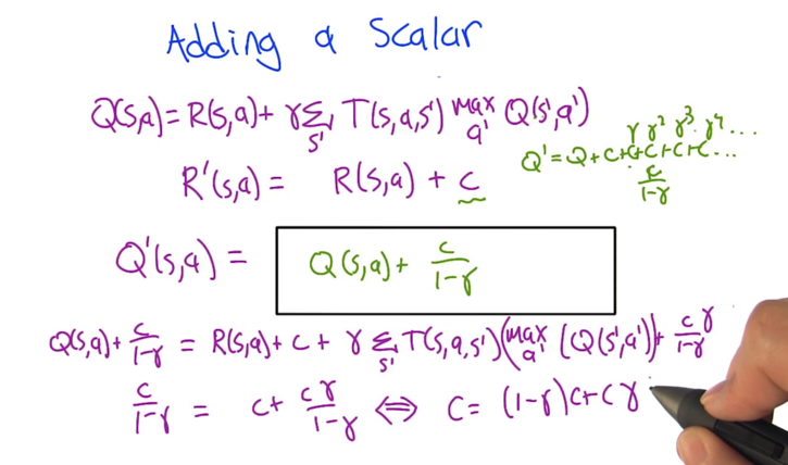
- Q = R + γR+γ2R + … + γ∞ R)
- Q’ = R’ + γR’+γ2R’ + … + γ∞ R’
- Replace R’ with R+c, Q’=(R+c) +γ(R+c)+γ2(R+c) + … + γ∞ (R+c) =(R + γR+γ2R + … + γ∞ R) + (c+γc+γ2c + … + γ∞ c)
- The first part is Q and the second part is geometric series. So, Q’ = Q + c/(1-γ)
3. nonlinear potential-based reward shaping
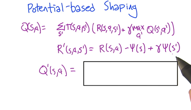
- Q = R + γR+γ2R + … + γ∞ R)
- Q’ = R’ + γR’+γ2R’ + … + γ∞ R’
- Replace R’ with R-ψ(s) + γψ(s’), Q’=(R-ψ(s) + γψ(s’)) +γ(R-ψ(s’) + γψ(s’’))+γ2(R-ψ(s’’) + γψ(s’’’)) + … + γ∞ (R-ψ(s∞ ) + γψ(s’∞ )) =(R + γR+γ2R + … + γ∞ R) + (-ψ(s) + γψ(s’) +γ(-ψ(s’) + γψ(s’’))+γ2(-ψ(‘’s) + γψ(s’’’)) + … + γ∞ (-ψ(s∞ ) + γψ(s’∞ ))
- The first part is Q. In the second part, most of the elements are cancelling each other out and only has the very first and last elements left. So, Q’ = Q + (-ψ(s) + γ∞ ψ(s’∞ )
- Given γ is in (0,1), so γ∞ =0. Then we have Q’: Q’ = Q - ψ(s)
Q-learning with potential
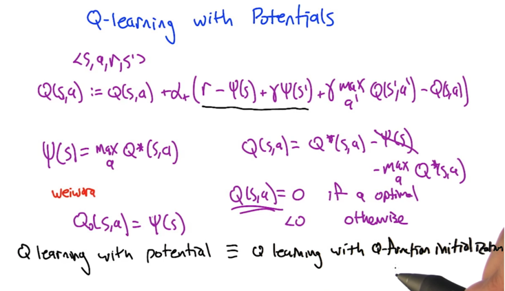
Updating the Q function with the potential based reward shaping,
- Q function will converge at Q*(s,a).
- we know that Q(s,a) = Q*(s,a) - ψ(s). If we initialize Q(s,a) with zero, then Q*(s,a) - ψ(s) = Q*(s,a) - maxaQ*(s,a) = 0, that means a is optimal.
- so Q-learning with potential is like initializing Q at Q*
What have we learned?
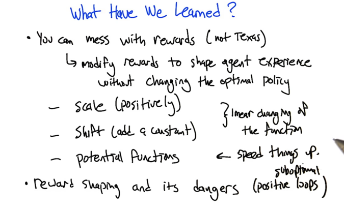
- Potential functions is a way to speed up the process to solve MDP
- Reward shaping might have suboptimal positive loops which will never converge?
2015-09-29 初稿
2015-12-04 reviewed and revised