This week
- Watch Generalization.
- The readings are Gordon (1995) and Baird (1995).
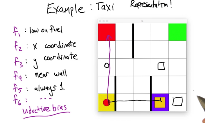
- When there are a lot of states, we can use features to represent states (e.g. grouping states using some common features or using some base states to represent other stats)
- Inductive bias: refer to the way algorithm prefer one solution against another.
- representation can stay unchanged even when states changed(?)
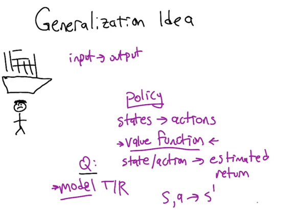
- In RL, the goal is to learn some input-output mapping.
- e.g. Policy maps state -> actions
- value function maps state/actions to expected return
- Model maps T/R (transition and reward)
- Generalization can happen on all these levels
- Most researchers are focused on value function approximation.
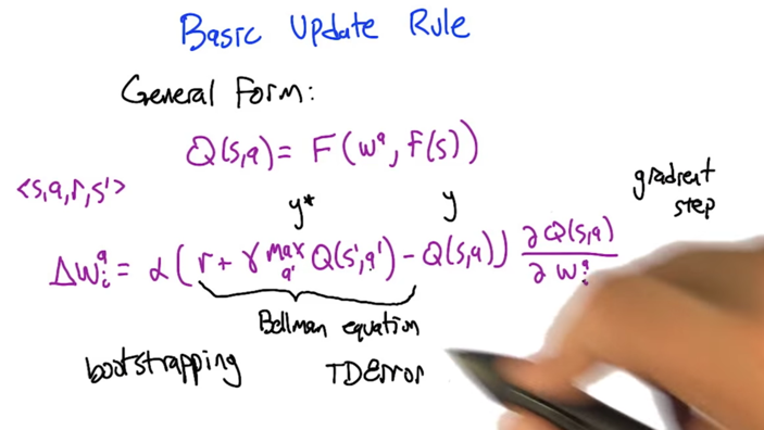
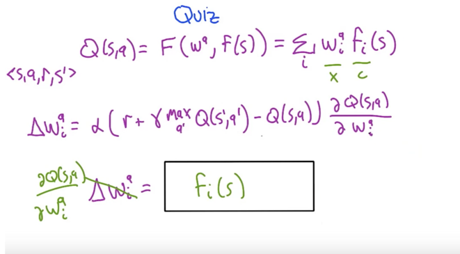
- Q is represented by function approximator F(wa, f(s)). wa is some kind of weights, f(s) takes a state s and generate a series of features.
- experience tuple <s,a,r,s’> comes in, and do an update.
- TD error= the difference between predicted value (reward + discounted value of next state) and value of current state. TD error tells us the direction to move the parameters w. (the prediction is high, low or just right).
- α is learning rate.
Linear Value Function Approximation
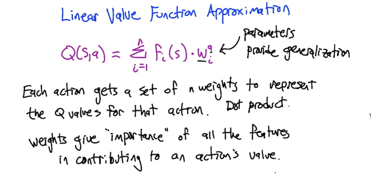
- Q value for an action is represented by features and a set of weights
- wai are weights of features fi(s), which represent importance of features
Success and fail stories
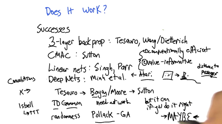
- 3-layer back prop: decision making in Jeopardy
- CMAC(wikipedia) :
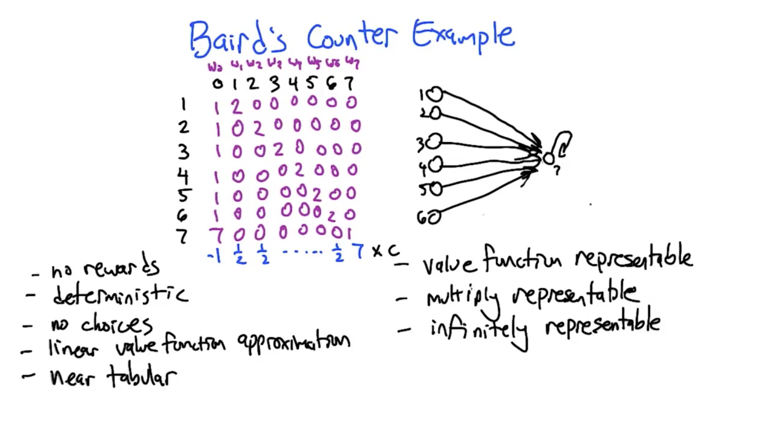
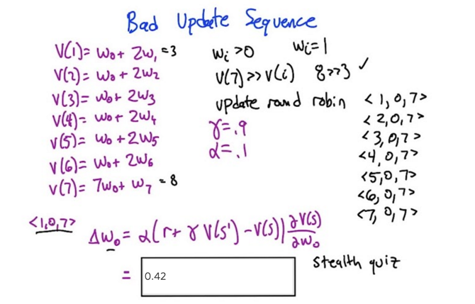
- V(s’) = V(7) =8; V(s) = V(1) =3, derivative is w =1; so Δw0 = 0.1( 0 + 0.9 * 8 -3)*1 = 0.42;
- Δw0 is 0.42, and Δwi, i = [0, 6] are all positive, so weight will increase with each update
-
Δw7 is negative when we update <7,0,7>, but w7 will still increase because it’s original value is » Δw7 - So, even the algorithm is doing the right thing, the updates will never converge
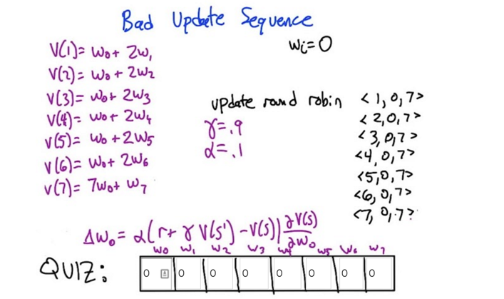
- in this case, the temporal differences are all zeroes because wi is 0, which means no updates (changes) are going to happen. Sticky
- If at any circumstance, when all values are zero, it could not escape the circumstance unless reward (r) is non-zero. If reward is also zero, we can call the circumstance the solution of the MDP.
- this holds when MDP is deterministic.
- the lesson: Shared weights can “not converge”!
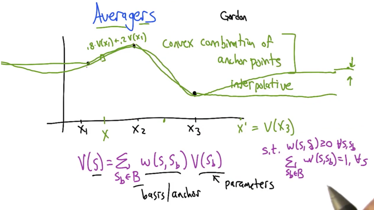
- Problem: given a certain points of value, estimate the function of line. How to estimates the points in-between?
- Naturally, weighted average of neighbours and get convex combinations of anchor points
- for points that are far from anchor points, are good estimate will be the average of the anchor points.
- more anchor points lead to less error in MDP estimation.
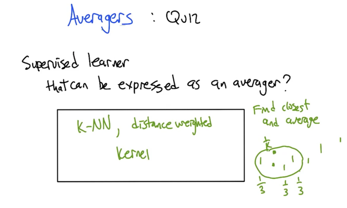
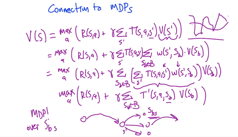
- Using base states, we can respresent the original MDP with MDP over Sbs
What have we learned
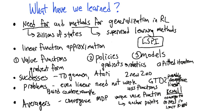
- Need for generalization: some problem have Zillions of states; Method: applying supervised learning method .
- Methods: Linear function approximation.
- 1) value functions 2) policies; 3) models;
- Success: TD gamma, Atari, Fitted Q-iteration (but still have need not work cases)
- Problem cases: even linear need not work (baird counter problem)
- Averagers: can be viewed as MDP itself. Use anchor points to represent the whole MDP.
- LSPI: Least Squared policy iteration
2015-10-13 初稿 upto quiz 1
2015-10-17 完成
2015-12-04 reviewed and revisted