- Temporal Abstraction Options
- Temporal Abstraction Option Function
- Pac-Man Problems
- How It Comes Together
- Goal Abstraction
- Monte Carlo Tree Search
- MCTS Properties
- Recap
This week
- watching Options.
- The readings are Sutton, Precup, Singh (1999) and Jong, Hester, Stone (2008) (including slides from resources link)


- Delayed reward: agent has weak feedback, the reward is a moving target
- Need exploration to learn the model or action-reward pair for all or a good number of states.
- computationally, the complexity of RL depends on number of states and # of Actions.
- Function approximation over value function (V(s), Q(s,a)) is abstraction over states, not actions.
- The focus of this class is abstraction over actions
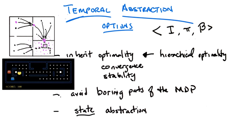
## Temporal Abstraction

- Original grid world problem: walls separated big square into four rooms, agent could be in any location. Agent’s actions are move L,R,U,D and its goal is to reach the small square in the bottom left room.
- a set of new actions (goto_doorway_X, X is orientation) can be generated to represent original actions.
- Temporal Abstraction is representing many actions with one or a few actions.(without doing anything to the states)
- Temporal Abstraction align many actions into on and thus makes a lot of states equivalent.
- Temporal Abstraction has computational benefits.
Temporal Abstraction Options
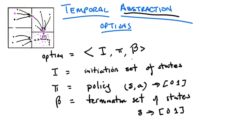
- Option is a tuple <I, π, β>
- I is initiation set of states
- π here is policy: probability of take action a in states s, (s,a) -> [0 1]
- β is termination set of states and it’s a set of probability of ending at state s, [0 1].
Temporal Abstraction Option Function
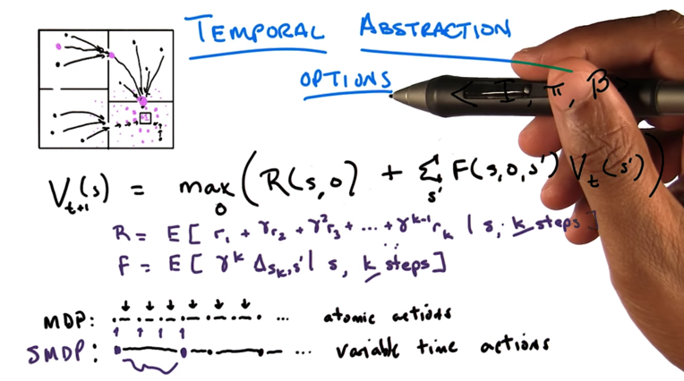
- The function is a rewrite of Bellman function
- using “o” to replace “a” (O is the generalization of A).
- V(s) ( and V(s’) ) is the value function that needs to update, R(s,o) is reward in s and choose a, F works like a transition function. the discount factor is hidden.
- Using options kind of violates the temporal assumption of MDPs
- MDPs have atomic actions, reward can be easily discounted for each step.
- Using options ends up with variable time actions, discount factor is hidden.
- If o represent k steps, R and F are actually discounted. this is Semi-MDP or SMDP
- we can turn non-Markovian stuff into Markovian by keep tracking of it’s history.
Pac-Man Problems
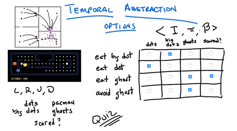
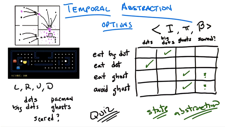
- We can learn two things from the example:
- If done improperly, temporal Abstraction might not reach optimal policy.
- temporal Abstraction might introduce state abstractions (reduce the state space) so the problem can be solved more efficiently.
How It Comes Together
- We can see options and state representations as high level representation. In fact, actions and states are also somewhat made up. Agent’s goal is to make decisions with respect to those descriptions of the world, no matter they are action or option, states or abstract states
- If construct options smartly, we might be able to ignore some states (decrease the state space) to reduce computational resource requirement.
Goal Abstraction
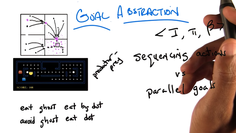
- agent has multiple parallel goals (predator-prey scenario ), at any given time, only one goal is dominating (more important).
- β (the probability of terminated in a state) can be seen the probability of accomplishing a goal or the probability of another goal becomes more important (switching goals).
- Options give ways to think actions as accomplishing parallel goals.
- The goals do not have to be in the same scale.
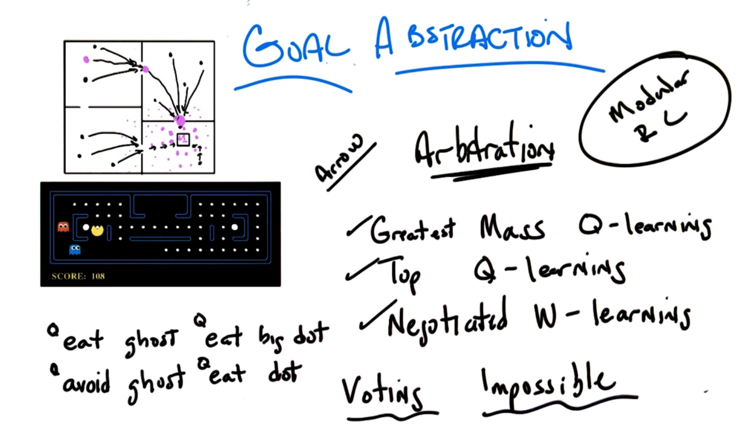
- Modular RL sees options as sub-agents with different goals. There are three ways of choosing goals:
- Greatest mass Q-learning: each action as a Q function. For each option, we sum up the Q functions of each action in it. The option with largest Q get executed. (might end up with agent with small Q on every action).
- Top Q-learnings: choose the action with highest Q. ( but the agent might put high Q on many actions)
- Negotiated W-learning: Minimize loss.
- Modular RL is often impossible because a fair voting system is hard to construct. e.g. the modules might have incompatible goals.
Monte Carlo Tree Search
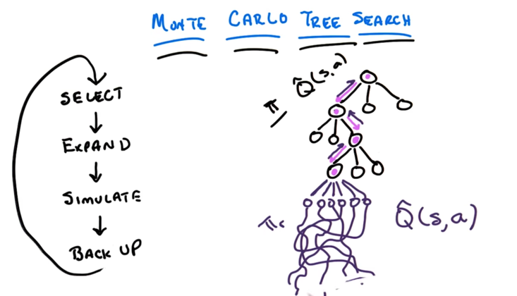
In the figure above, circles are states, edges are transitions. π =Q^(s,a) is the policy of the known part of the tree. In these states, we know what action to take following π (pink edges). When reach an unknown state, we apply the rollout policy πr, and simulate actions to take deep in the tree, and then we backup and update πr and π to figure out what to select at each state, including the unknown state where we started the simulation. π gets expanded as we figure out the policy at unknown state. Then repeat the “Select, Expand, simulate, back up” process.
- initial policy π, we can SELECT actions following it. it can be updated at each iteration of tree search.
- rollout policy πr, we can simulate actions and sample from them starting from the unknown state following it.
- we back up after stimulation with the simulated result to update π.
- we figured out what action to take at the unknown state and states above and expand π to the previous unknow state.
- now we can repeat the process to search deeper.
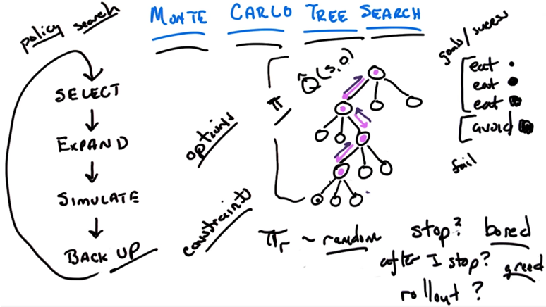
- when to stop? learn deeper enough before reach the computational resource cap
- rollup policy πr can be random. we know the action is good because I get better result by behaviouring randomly from that point on.
- instead of purely random, on can behave randomly in respect to constraints. (e.g. not eaten by ghost).
- constraints: defined by failure
- goals: defined by success
- MCTS is compatible with options to perform the tree search. in this case, π = Q_hat(s,o);
- the Monte Carlo Tree Search can be seen as policy search. When reach a state we are not confident, a inner loop is executed to do some RL.
MCTS Properties
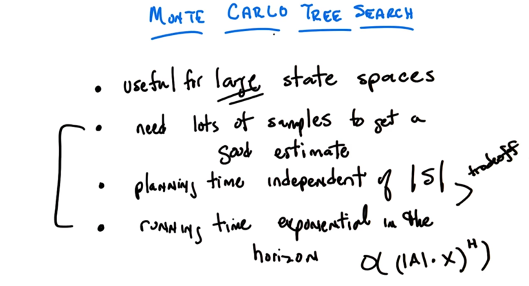
- MCTS is useful for large state spaces and need lots of sample s to get good estimates
-
Planning time is independent of S -
Running time is O( ( A .X)H ). - X is how many steps does the search need to go through
-
A is the size of the action space
- The tradeoff is between number of states and how far away are we going to search
Recap

2015-10-28 初稿
2015-11-01 finished.
2015-12-04 reviewed and revised