Week 05 tasks
- Lectures: the remainder of Bayesian Learning and Inference.
- Reading: Chapter 6 of Mitchell.
SL10: Bayesian Inference
Intro
- About these probabilistic quantities that we’re working with, Is there anything that we need to know about how to represent and reason with them.
- Bayesian Networks, which is this wonderful representation for representing and manipulating probabilistic quantities over complex spaces.
Joint Distribution
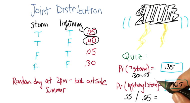
- build on this idea of a joint distribution.
- The probability of not have a storm and the the probability of lightning given there is a strom.
Adding Attributes
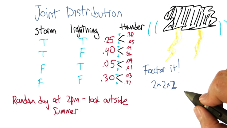
- each time we add one variable, the number of probabilities that we have to write down will go up as factor of two
- factor it: instead of representing all as eight numbers, we can represent it by 2 times 2 time 2.
Definition for conditional independence
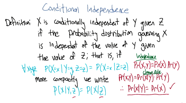
- conditional independence: the probabilities associated with the values in this variable X Is independent of the value of y given the value of z.
- if we know z, then the probability of x can be figured out without knowing y.
- normal independence: Pr(x,y) =Pr(x)Pr(y) *the chain rule: Pr(x,y) =Pr(x|y)Pr(y)
-
So that means: Pr(x y) = Pr(x). - conditional independence gives us: As long as there is some z that we stick in here, that gives us that property that we can essentially ignore y, when we are talking about the probability of x.
- We are factoring that probability distribution
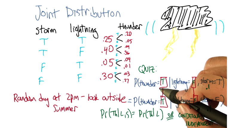
- find a truth setting for thunder and lightning, such that the probability that thunder takes on that value, given that lightning takes on the value that you give, and the storm is true, ends up equaling the probability that thunder takes on that value given lightning takes on the value that you gave and storm is false. so a setting here so that basically the value of storm doesn’t matter.
- No matter what you put in here, the answer will be correct. Why? because Storm doesn’t matter.
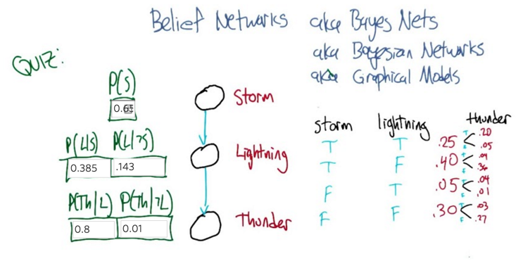
- figuring out those probabilities is really easy
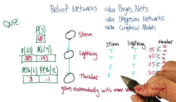
- the probability depends on the connections between nodes and it can grow exponentially with more variables.
Sampling From The Joint Distribution
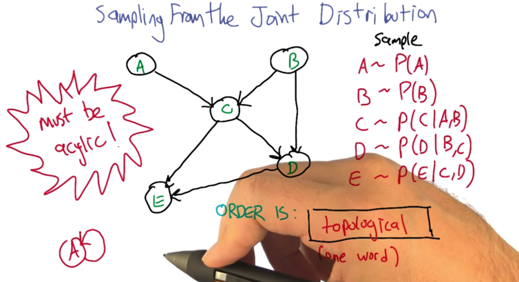
- topological sort: a standard thing that you can do with a graph, and it’s very quick.
- The graph must be a directed acyclic one: you can’t have arrows that take you back.
.
Recovering the Joint Distribution
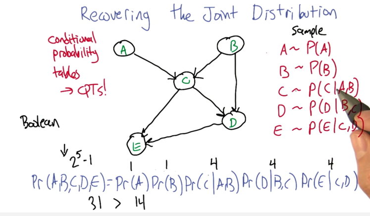
- recover the joint distribution
- and that’s much more compact a representation ( sing 14 numbers instead of 31 numbers)
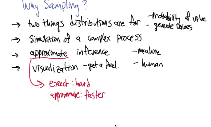
- With a distribution you can
- tell the probability of a certain value
- generate values according to that distribution.
- Simulate the distribution. A distribution represents kind of a process, we could duplicate that process by sampling
- approximate inference: get a sense how the data is by sampling- machine
- Visualization - to get feel of the data - human sense.
Inferencing Rules
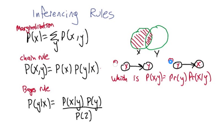
- marginalization: representing the probability of x by summing over some other variable y and looking at the joint probabilities of those. e.g.
P(x) = P(x|y=true) +P(x|y=false) -
The chain rule: P(x,y) = P(x)p(y x)=p(y)p(x y) -
Bayes rule: p(y x)=P(x y)P(y)/P(x) -
question: which tree represents P(x,y) = p(y)p(x y). - These three together could work out the probability of various kinds of events.
Inference By Hand
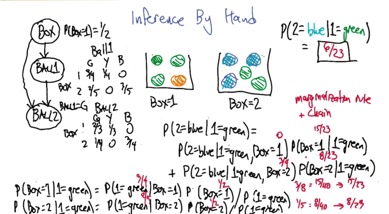
- example: 2 boxes with balls in it. Question: what’s the probability of drawing a blue ball given that we get a green ball in box 1.
- need to apply the marginalization, the chain rule and the bayes rule to break the first probability down.
-
then use the bayes rule to calculate and normalize P(box=1 1=green) and P(box=2 1=green).
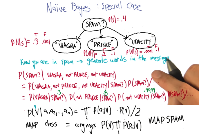
- in the spam classification problem. bayes rule can be used to map class from attributes.
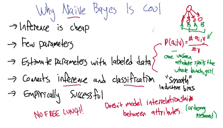
- it assumes that all the attributions are conditional independent
2016-02-10 stopped at "Recovering the Joint Distribution"
2016-02-11 初稿完成