- 01 - Overview
- 02 - What is Q
- 03 - Learning Procedure
- 04 - Update Rule
- 05 Update Rule
- 06 - Two Finer Points
- 07 - The Trading Problem - Actions
- 08 - The Trading Problem: Rewards
- 09 - The Trading Problem: State
- 10 - Creating the State
- 12 - Discretizing
- 13 - Q-Learning Recap
- Summary
- Resources
01 - Overview
- Q-learning is a model-free approach. The transitions T or the rewards R are unknown.
- Q-learning builds a table of utility values as the agent interacts with the world.
- These Q-values can be used at each step to select the best action based on what it has learned so far.
- Q-learning guaranteed to provide an optimal policy. There is a hitch, however, that we’ll cover later.
Time: 00:00:38
02 - What is Q
What is Q?
Well, let’s dig in and find out.
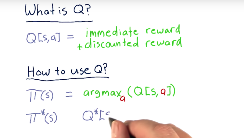
- in this class we’re going to view Q as a table with two dimensions, s and a.
Q[s, a]Q represents the value of taking action A in state s.- two components: the immediate reward that you get for taking action A in state s, plus the discounted reward or the reward you get for future actions.
- Q is not greedy: it just represents the reward you get for acting now and the reward you get for acting in the future.
How can we use Q to figure out what to do?
Policy ($\Pi$) defines what we do in any particular state
- $\Pi(s)$ is the action we take when we are in state s.
- $\Pi(s) = argmax_a(Q[s, a])$, So we step through each value of a, and the one that is the largest is the action we should take.
After we run Q learning for long enough, we will eventually converge to the optimal policy ($\Pi^*$).
Time: 00:02:53
03 - Learning Procedure
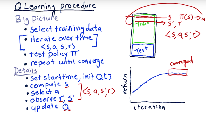
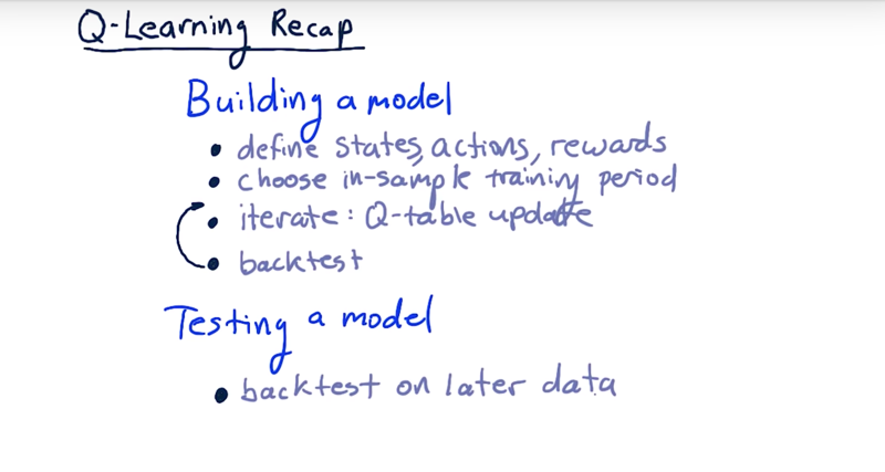
the big picture of how to train a Q-learner.
- select data to train on: time series of the stock market.
- iterate over this data over time. Evaluate the situation there and for a particular stock that gives us s our state. consult our policy and get an action a. take that action, evaluate the next state s’ and our reward r. that is <s, a, r, s’>, the experience tuple.
- Once get all the way through the training data, test our policy and see how well it performs in a backtest. 4 If it’s converged or it’s not getting any better then we say we’re done. If not, repeat this whole process all the way through the training data.
what does converge mean?
As we cycle through the data training our Q table and then testing back across that same data, we get some performance. And we expect performance to get better and better.
- But after a point, it finally stops getting better and it converges. When more iterations don’t make performance better and we call it converged at that point.
Detail on what happens here when we’re iterating over the data.
- start by setting our start time, and initialize our Q table.
- The usual way to initialize a Q table is with small random numbers, but variations of that are fine.
- observe the features of our stock or stocks and from those build up together our state
s. - consult our policy (Q table) to find the best action in the current state to get
a. - step forward and get reward
rand new states'. - Update the Q table with this complete experience tuple
Then repeat.
Time: 00:03:22
04 - Update Rule
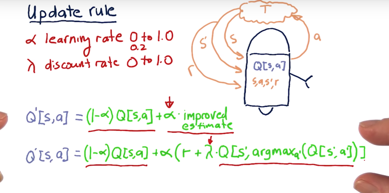
Once an experience tuple <s, a, r, s’> is generated by interacting with the environment, how does it take that information to improve this Q table?
There are two main parts to the update rule.
- the old value that we used to have: Q [s, a].
- improved estimate
Learning Rate: New concept: $\alpha$ is the learning rate. $\alpha \in [0,1]$, usually use about 0.2.
- $Q’[s,a] = ( 1 -\alpha)Q[s,a] + \alpha * \text{estimated improvement})$
- This learning rate dictates the ratio the Q’ takes from the old Q and the estimated improvement.
- larger values of $\alpha$ cause us to learn more quickly, lower values of $\alpha$ cause the learning to be slower.
- a low value of alpha, for instance, means that in this update rule, the previous value for Q[s,a] is more strongly preserved.
Discount rate $\gamma$ is the discount rate. $\gamma \in [0, 1]$. A low value of $\gamma$ means that we value later rewards less.
- A low value of $\gamma$ equates to essentially a high discount rate.
- The high value of $\gamma$, in other words, a $\gamma$ near 1, means that we value later rewards very significantly.
- $Q’s,aQ[s,a] + \alpha( r + \gamma Q[s’,argmax_{a’}(Q[s’,a’])$
future discounted rewards.
what is the value of those future rewards if we reach state s’ and we act appropriately?
- Q value, but need to find out what the action to take. which is $argmax_{a’}(Q[s’,a’]$
This is the equation you need to know to implement Q learning.
Time: 00:05:07
05 Update Rule
The formula for computing Q for any state-action pair <s, a>, given an experience tuple <s, a, s', r>, is:
Q'[s, a] = (1 - α) · Q[s, a] + α · (r + γ · Q[s', argmaxa'(Q[s', a'])])
Here:
r = R[s, a]is the immediate reward for taking actionain states,γ ∈ [0, 1](gamma) is the discount factor used to progressively reduce the value of future rewards,s'is the resulting next state,argmaxa'(Q[s', a'])is the action that maximizes the Q-value among all possible actionsa'froms', and,α ∈ [0, 1](alpha) is the learning rate used to vary the weight given to new experiences compared with past Q-values.
06 - Two Finer Points
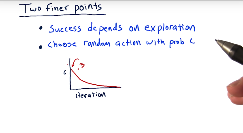
- Q-learning depends to a large extent on exploration. So we need to explore as much of the state and action space as possible.
Randomness.
- where we are selecting an action, we flip a coin and randomly decide if we’re going to randomly choose an action.
Two flips of the coin. 1) choose a random action or are action with the highest Q value? 2) if random choice, then flip the coin again to choose which of those actions we’re going to select.
- A typical way to implement this is to set this probability at about 0.3 or something at the beginning of learning * And then over each iteration to slowly make it smaller and smaller and smaller until eventually we essentially don’t choose random actions at all.
By doing this,
- we’re forcing the system to explore and try different actions in different states.
- it also causes us to arrive at different states that we might not otherwise arrive at if we didn’t try those random actions.
Time: 00:01:32
07 - The Trading Problem - Actions
To turn the stock trading problem into a problem that Q learning can solve, we need to define our actions, we need to define our state, and we also need to define our rewards.
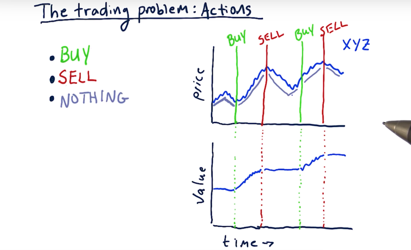
Actions.
Three actions, buy, sell or do nothing.
Usually what’s going to happen most frequently is that we do nothing.
- So we evaluate the factors of the stock (e.g. several technical indicators) and get our state.
- We consider that state and we do nothing for a while
- something triggers an buy action: So we buy the stock and holding 4. then do nothing until our very intelligent Q learner says otherwise.
How this sort of stepped behavior affect our portfolio value
Time: 00:02:22
08 - The Trading Problem: Rewards
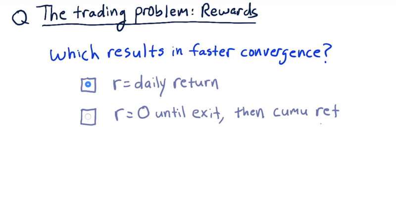
Now consider rewards for our learner: 1)Short-term rewards in terms of daily returns or 2) long-term rewards that reflect the cumulative return of a trade cycle from a buy to a sell, or for shorting from a sell to a buy.
Which one of these do you think will result in faster conversions? Solution: The correct answer is daily returns.
Daily returns give more frequent feedback while cumulative rewards need to wait for a trading cycle to end.
Time: 00:00:41
09 - The Trading Problem: State
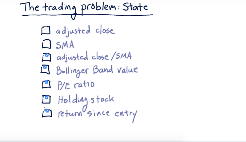
Which of the indicators are good candidates for states?
Solution: Adjusted close or SMA are not good factors for learning, not able to generalize over different price regimes for when the stock was low to when it was high. but the combine adjusted close and simple moving average into a ratio that makes a good factor to use in state.
Bollinger Band value, P/E ratio is good.
holding the stock or not: is important to the actions. return since we entered the position might be useful to determine the exit points
Time: 00:01:34
10 - Creating the State
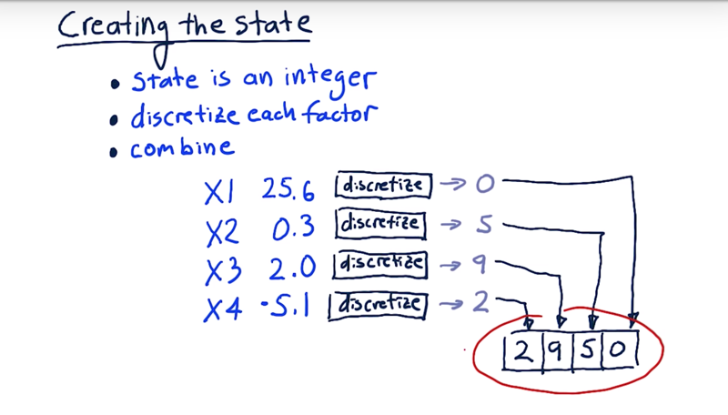
The state is a single integer so that we can address it in our cue table. We can 1) discretize each factor and 2) combine all of those integers together into a single number.
-
For example, we have four factors and each one is a real number. Then we discretize each one of these factors.
-
So we run each of these factors through their individual discretizers and we get an integer.
Now we can stack them one after the other into our overall discretized state.
Time: 00:01:52
12 - Discretizing
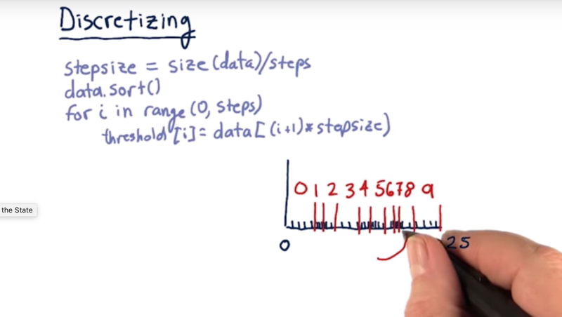
Discretization or discretizing: convert a real number into an integer across a limited scale.
- the number of steps we’re going to have.
- divide how many data elements we have all together by the number of steps.
- Then we sort the data, and then the thresholds just end up being the locations for each one of these values.
Time: 00:01:53
13 - Q-Learning Recap
Total Time: 00:24:12
Summary
Advantages
- The main advantage of a model-free approach like Q-Learning over model-based techniques is that it can easily be applied to domains where all states and/or transitions are not fully defined.
- As a result, we do not need additional data structures to store transitions
T(s, a, s')or rewardsR(s, a). - Also, the Q-value for any state-action pair takes into account future rewards. Thus, it encodes both the best possible value of a state (
maxa Q(s, a)) as well as the best policy in terms of the action that should be taken (argmaxa Q(s, a)).
Issues
- The biggest challenge is that the reward (e.g. for buying a stock) often comes in the future - representing that properly requires look-ahead and careful weighting.
- Another problem is that taking random actions (such as trades) just to learn a good strategy is not really feasible (you’ll end up losing a lot of money!).
- In the next lesson, we will discuss an algorithm that tries to address this second problem by simulating the effect of actions based on historical data.
Resources
- CS7641 Machine Learning, taught by Charles Isbell and Michael Littman
- Watch for free on Udacity (mini-course 3, lessons RL 1 - 4)
- Watch for free on YouTube
- Or take the course as part of the OMSCS program!
- RL course by David Silver (videos, slides)
- A Painless Q-Learning Tutorial
2019-03-31 初稿