- Challenge Question
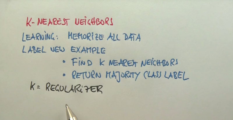
- k-Nearest Neighbors
- Cross Validation
- K As Smoothing Parameter
- The Gaussian Distribution
- Bayes Classifier
- Decision Tree
- Random Forest
This week: watch the first section of Lesson 7, Machine Learning (through Random Forests), and read Chapters 18.1-5, 18.8, 20.1-20.2 in AIMA (Russell & Norvig).
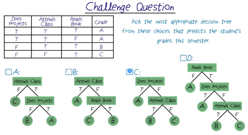
Challenge Question
Find the most efficient decision tree given the fact table
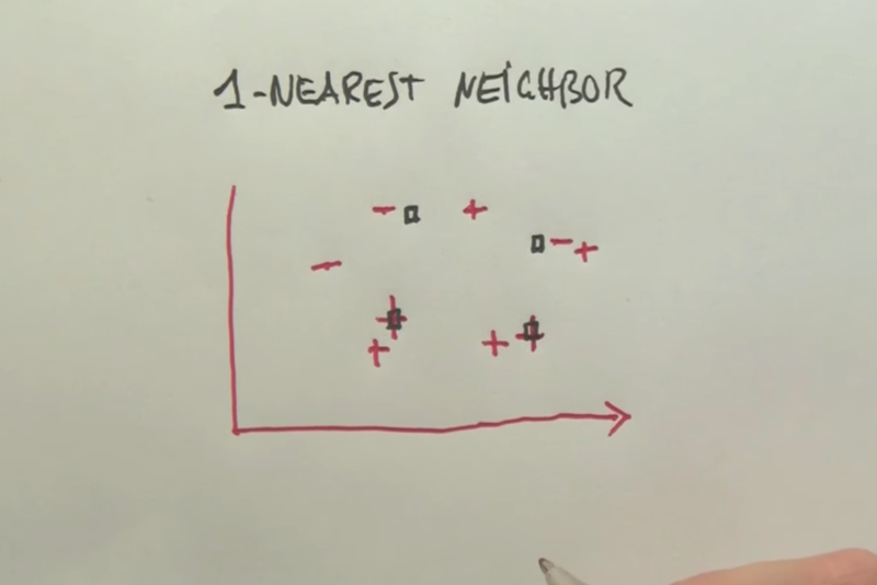
k-Nearest Neighbors
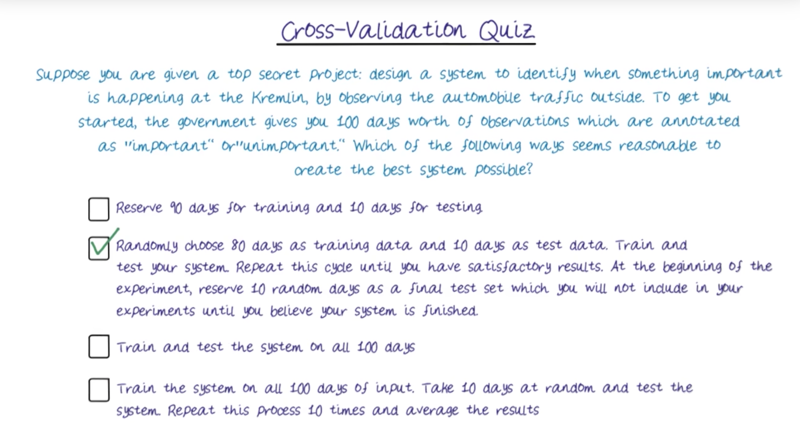
Cross Validation
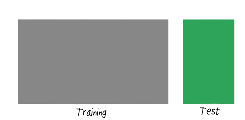
- Training set and test set. Cross-validation often uses a randomly chosen independent sample as test sets.
- Model selection: tweaking parameters of the model and report the one which gives the best prediction ( be this might lead to the over-fitting problem.
- Leave-one-out cross-validation (LOOCV) strategy: when a sample is small, a test set might not be feasible, in this case, use the leave-one-out strategy in which we train the model with all cases in a data set except one random case. repeat the process multiple times with one case leave out.
AIMA: Chapter 18.8 Further study: Sebastian Thrun’s and Peter Norvig’s lecture on kNN
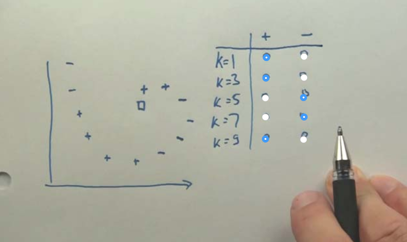
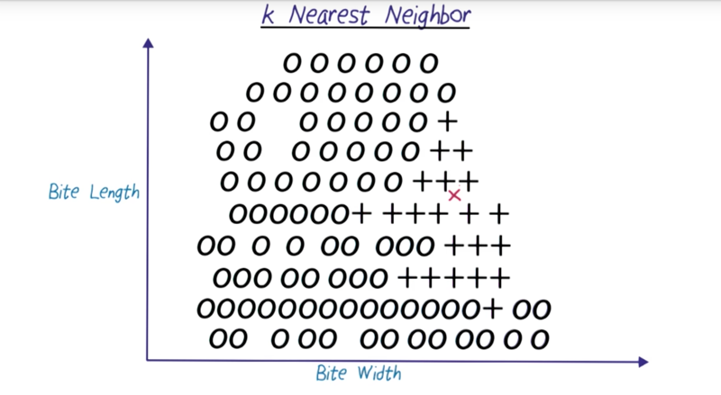
- which data point is positive given the known data points?
- what is the value of the data points using kNN when k = 1, 3, 5, 7, 9?
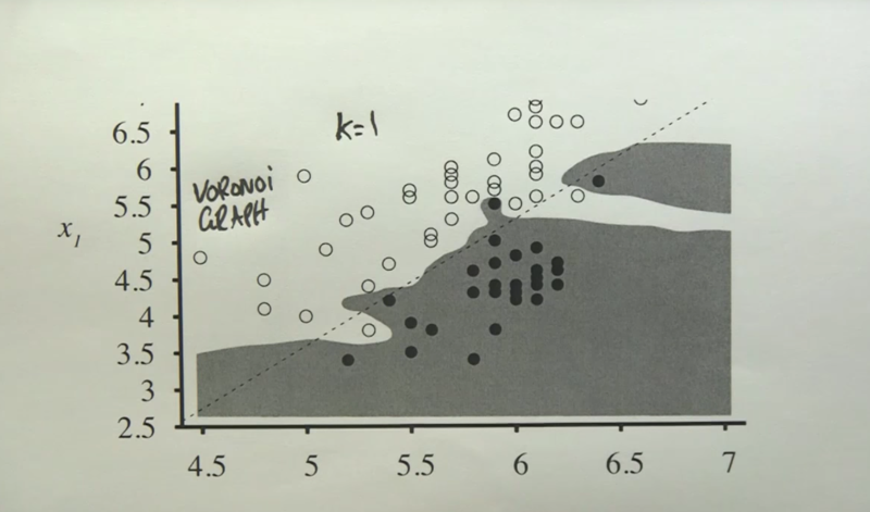
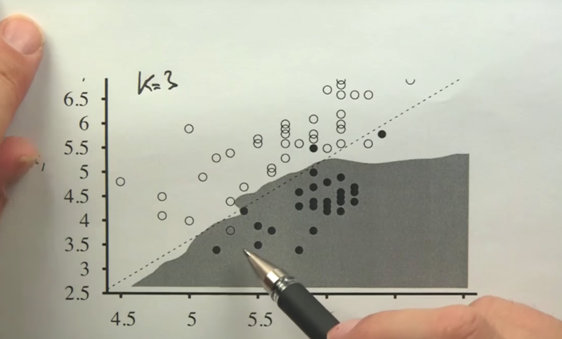
K As Smoothing Parameter
- as K increases, the separation boundary becomes smoother, but there are more outliers which will be misclassified. The model will also be come more complex
The Gaussian Distribution
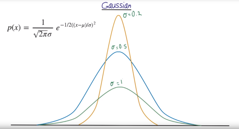
- standard deviation determines the width of the distribution
- 68% with 1 SD, 95% within 2 SD, 99.7% with 3 SD.
Central Limit Theorem
- Samples of random variables, the mean of the samples will form a Gaussian Distribution. And the mean of the distribution will be expected to be the population mean
Grasshoppers Vs Katydids
A pattern recognition example of Gaussian distribution
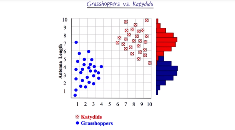
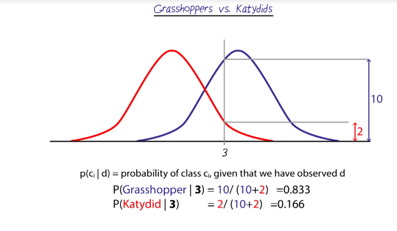
- the distribution can be formed by projecting data on to the Y-axis.
- once a distribution is formed, it is very easy to get the probability of what a case if from by fit it in the distribution.
Quiz: Gaussian Distribution
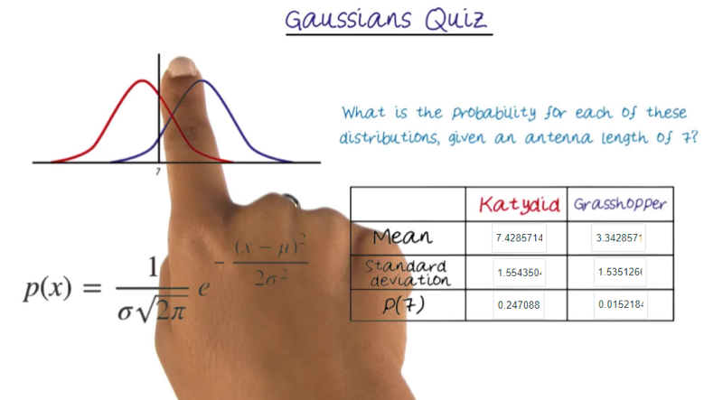
Take the Insect data: Antennae length [xlsx | csv] and calculate the probability of the length “7” indicate a Katydid or Grasshopper
Decision Boundaries
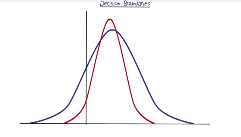
- the boundary is where the distributions cross.
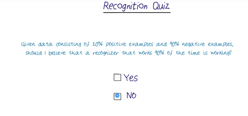
- “No” because the recognizer might classify everything as negative and get 90% cases correctly.
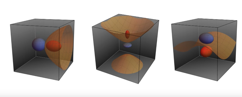
Decision Boundaries in Higher Dimensions
- The Decision boundaries are also in higher dimensions for higher dimensional distribution
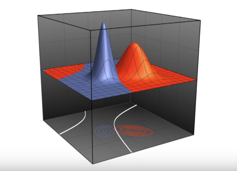
Error
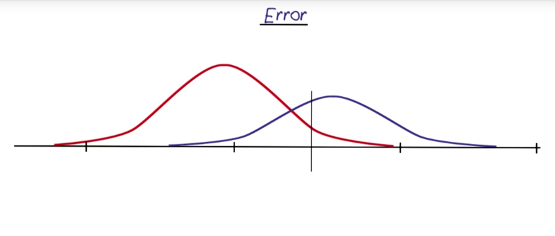
- we can make the decision boundary which changes the error rate of the classification. In real life, the decision should be made to increase acceptable errors (classify mosquitoes don’t care certain disease as the ones who carry the disease) to avoid unacceptable errors (misclassify bad as good).
Bayes Classifier
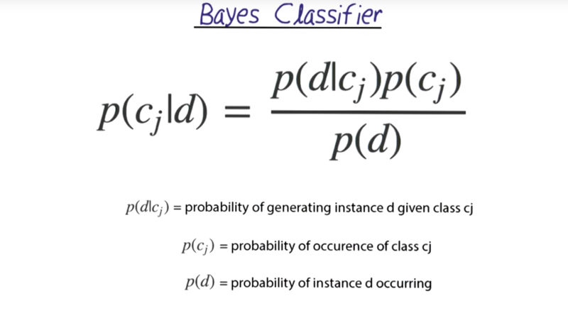
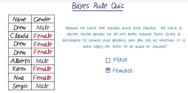
-
based on the table P(G N ) = P(N G) * P(G)/P(N) - using counting to get the probabilities. E.g. P(male), there are 3 males in 8 data points, then p(male) = 3/8, etc…
- N = Name = Drew here.
-
P (male Drew)= P(Drew male) P(male) /P(Drew) = 1/3 * 3/8 / (3/8) = 0.33 -
P (female Drew)= P(Drew female) P(female) /P(Drew) = 2/5 * 5/8 /(3/8) = 10/15 = 0.67
Naive Bayes
- Independent assumption gives Naive Bayes.
- Naive Bayes can be represented as a tree structure of class pointing to features
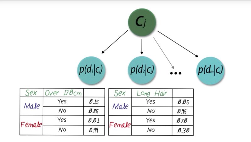
Naive Bayes net assumes independence between features: so P( height, hair length | sex) = P(height | sex) * P(hair length | sex), thus
-
p(d Cj) = p(d1Cj) * p(d2Cj) * … * p(dmCj) - here we assume Maximu Likelihood where everyone prior has the same probability of occurence.
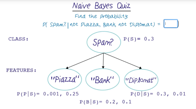
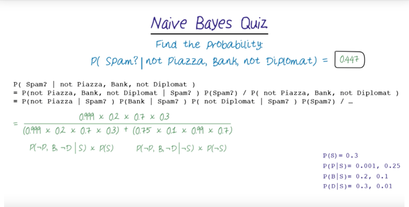
Readings for Bayesian Classifiers
- AIMA: Chapter 20.1-20.2
Further resources
No Free Lunch
No one ML algorithm is good for all problems.
Naive Bayes vs kNN
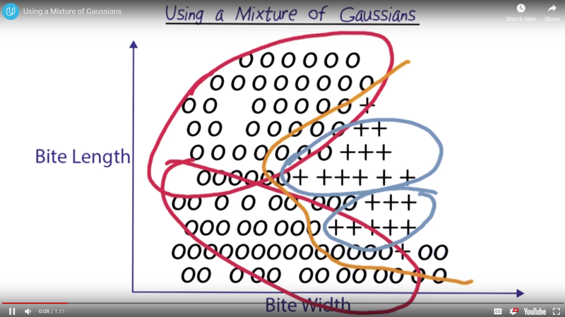
using a mixture of Gaussians
-
Two Gaussian can generate a more complex decision boundary, and more Gaussian can do more until it creates its own decision boundaries for each of the data points which is nearly the same as kNN.
- Kernel density estimation: use fewer Gaussians which would cause the decision boundary to be smooth, But still give a good continuous approximation of the shape
- cross-validation can be used to find the good N of Gaussians.
- use a final test set to test for overfitting.
Generalization
Visualization
Visualize data to determine which algorithm might work.
- If most of the classes from balls of data without many concavities, then modeling it with Gaussians will probably work well.
- If there are situations where classes interpenetrate, but still have distinct boundaries, then k-nearest neighbors or one of the kernel methods will probably work.
- for high dimensional data we can also use methods like decision trees and boosting to help you understand which features are most important.
Decision Tree
Decision tree with discrete information
Decision tree with continuous information
Minimum Description Length
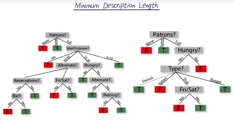
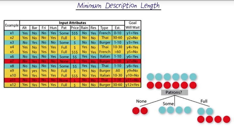
- which attributes should we use first?
- Which question provides the most solution of the problem? then it should be on the top of the decision trees according to information theory.
Entropy
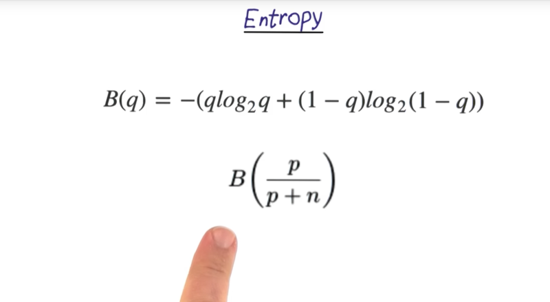
- p is the number of positive cases
- n is the number of negative cases
- B(q) = -(qlog2q + (1 - q)log2(1 - q))
Information Gain
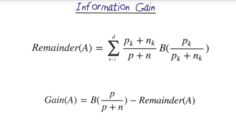
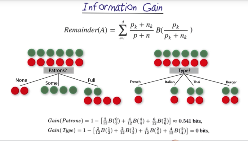
- Information Gain is a way to determine how to construct three
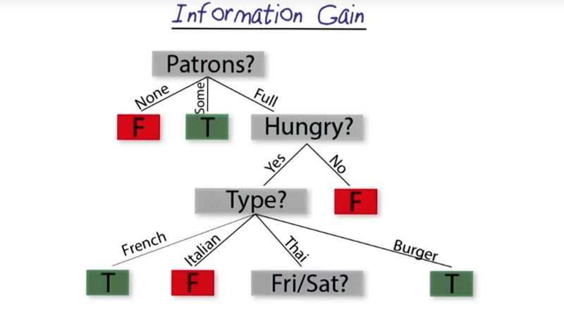
- Please note that the attribute which is not important at the first iteration might become important in the new level.
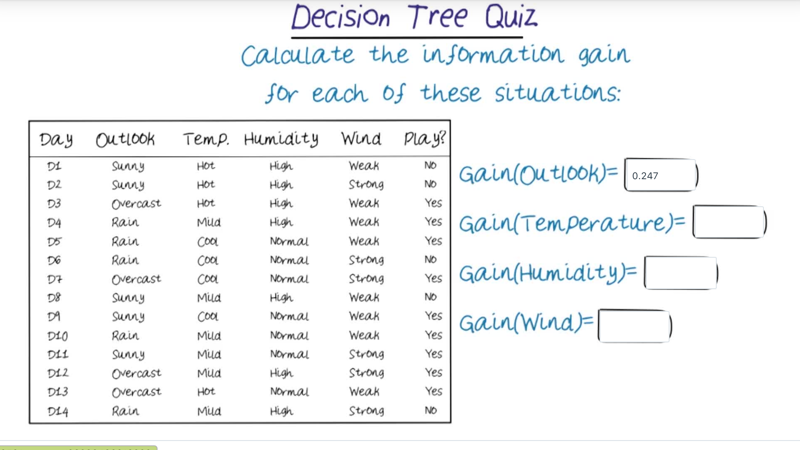
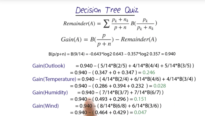
- B(9/14) = 0.94 Gain(outlook) = 0.94 - [5/14 * B(3/5) + 4/14 * B(4/4) + 5/14 * B(2/5)] =0.94 - [5/14 * 0.97 + 5/14 * 0.97]
Readings on Decision Trees
AIMA: Chapter 18.1-18.5
Random Forest
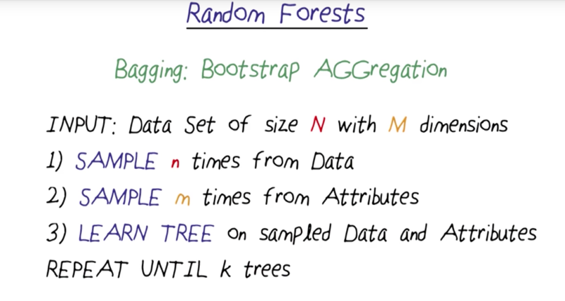
- train several decision trees and let them vote for the answer
- Random sampling seems to be able to lower the chance of overfitting
week 09 is the midterm week. No lectures
